Understanding LLM Inference Through Nano-vLLM
11 Apr 2026Nano-vLLM is a lightweight vLLM implementation built from scratch in ~1,200 lines of Python. It achieves comparable inference speed to vLLM while remaining readable end-to-end. This post walks through the architecture, answers common questions about how the key systems work, and profiles the engine on Qwen3-4B to see where the time actually goes.
- Why Nano-vLLM Is Worth Studying
- Understanding the Architecture: Q&A
- How does continuous batching work?
- How does paged KV cache and prefix caching work?
- How does the attention context work?
- How does tensor parallelism synchronize across ranks?
- Why RMSNorm instead of LayerNorm?
- How does the Triton KV store kernel work?
- What are the Flash Attention API conventions?
- What are CUDA graphs and what can they capture?
- PyTorch aside: broadcasting vs indexing alignment
- Profiling Experiments
Nano-vLLM is an offline inference engine — you hand it a list of prompts, it processes them in batches, and returns all results when done. It is not a serving system. There is no HTTP/gRPC server, no request routing, no streaming — generate() returns only after every sequence has finished (nanovllm/engine/llm_engine.py:89).
What it does implement: the core compute and memory systems that make LLM inference fast — paged attention, continuous batching, prefix caching, CUDA graphs, tensor parallelism, and torch.compile. What it doesn’t:
- No server — no HTTP/gRPC/OpenAI-compatible API, no authentication, no request IDs
- No online request handling — no async queue, no cancellation, no disconnect handling, no backpressure
- No streaming — tokens are returned only after the full sequence completes
- No speculative decoding — no draft model or verification
- No disaggregated prefill/decode — prefill and decode share the same GPU
- No quantization — weights are full precision (BF16), no INT8/INT4/FP8
- No multi-model / multi-LoRA — single model, no adapter swapping
- Single node only — tensor parallelism across GPUs on one machine, no multi-node
These are important for production, but not essential for understanding how the core inference engine works — which is exactly the point.
Why Nano-vLLM Is Worth Studying
The vLLM source code is a maze — hundreds of files, layers of abstraction, and config options for every conceivable deployment scenario. Nano-vLLM strips all of that away and keeps the core ideas intact:
- Paged Attention with a block manager and KV cache (~153 lines)
- Continuous Batching with a prefill-first scheduler (~85 lines)
- Prefix Caching via content-based hashing with xxhash
- CUDA Graphs for decode with pre-allocated tensors (~60 lines)
- Tensor Parallelism with column/row-parallel linears and shared-memory IPC
- torch.compile on RoPE, RMSNorm, SiluAndMul, and the sampler
- Custom Triton kernel for KV cache store operations
The entire engine — scheduler, block manager, model runner, sequence tracking — fits in ~500 lines. Each file is small enough to read in one sitting. For understanding how LLM inference engines work, this is the codebase to start with.
Currently only Qwen3 is supported (a dense decoder-only transformer, not MoE). The plumbing is generic enough that adding another decoder-only family (Llama, Mistral, Gemma) would be straightforward, but there’s no plug-and-play multi-model support. Tensor parallelism is local-only (single node, multiple GPUs).
Key Classes
-
Sequence— per-request state:token_idsandblock_table(list of physical block IDs mapping this sequence’s logical blocks to GPU KV cache pages). -
BlockManager— maintains a pool of KV cache blocks. Assigns blocks to sequences (which become theirblock_table), tracks ref counts, and manages prefix cache lookups. -
Scheduler— returns a list ofSequences to run each step. Prefill-first from the waiting queue; decode batches are reassembled every step from the left side of the running queue. Sequences finish and leave; new ones enter. Continuous batching here is simple because the working set is rebuilt each step. -
LLMEngine— createstp_sizenumber ofModelRunnerprocesses (each with a separatemp.Event), loops schedule → run → postprocess steps until every sequence is done. -
ModelRunner— owns the model shard and KV cache on one GPU. Rank > 0 workers sit in a command loop; rank 0 drives. Method calls are synchronized viaEventand passed viaSharedMemory(pickled). Key details:- KV cache tensor shape:
(2, num_layers, num_blocks, block_size, num_kv_heads, head_dim) prepare_prefill: only processes non-prefix-cached tokens — concatenates them across all sequences into flatinput_ids. Positions andslot_mapping(physical KV cache write addresses) are built similarly. The slot table itself contains all slot IDs, cached or not.prepare_decode: simpler — just the last token of each sequence.- Input to the model is shaped
[num_new_tokens]— there is no batch dimension.
- KV cache tensor shape:
System Diagram
+-----------------------------------------------+
| User Python Process                           |
|   LLM / LLMEngine                             |
|     ├── AutoTokenizer                         |
|     ├── Scheduler ── BlockManager             |
|     └── rank 0 ModelRunner                    |
|          ├── Qwen3 model shard                |
|          └── KV cache on GPU 0                |
+-----------------------------------------------+
                      |
                      | torch.multiprocessing (spawn)
                      | + shared memory + Event
                      v
+---------------------+  +---------------------+
| TP Worker (rank 1)  |  | TP Worker (rank 2)  |
|  ModelRunner.loop() |  |  ModelRunner.loop()  |
|  Qwen3 model shard  |  |  Qwen3 model shard  |
|  KV cache on GPU 1  |  |  KV cache on GPU 2  |
+---------------------+  +---------------------+

All ranks join one local NCCL process group.
Request Flow
prompt(s)
  → tokenize in main process
  → Sequence objects
  → Scheduler.schedule()
      - prefill new requests from waiting queue, or
      - decode running requests from running queue
  → rank 0 ModelRunner.call("run", ...)
      → if TP > 1: send same command to worker ranks via shared memory
      → all ranks run forward pass (NCCL all_reduce synchronizes)
      → rank 0 samples next token ids
  → Scheduler.postprocess()
  → when finished: main process decodes token ids to text
Understanding the Architecture: Q&A
How does continuous batching work?
The scheduler maintains two queues: a waiting queue for sequences that need prefill, and a running queue for sequences in the decode phase. Each step, the scheduler first drains the waiting queue (prefill-first priority), then decode batch is assembled from the left side of the running queue up to the batch size limit every step. A prompt will finish decode unless preempted, which happens at right side of running queue.
Even though this is offline inference (all prompts submitted upfront), the scheduler is still essential — if 1000 prompts come in, the engine may only process 16 or 64 at a time, rotating and admitting more as GPU memory and batch limits allow. New sequences enter decode as earlier ones finish, keeping the GPU busy.
When memory runs low, the scheduler preempts the most recently added decode sequence — deallocates its blocks and pushes it back to the waiting queue for re-prefill. The preempted sequence’s KV cache is logically released (not preserved), so it recomputes from the beginning when rescheduled. Simple and correct, no complex eviction policies.
One limitation: prefill and decode are never mixed in the same batch. Each step is either all-prefill or all-decode.
Thread safety: The engine is not thread-safe. The safe pattern is one engine instance, one caller at a time, and pass many prompts in a single generate() call.
How does paged KV cache and prefix caching work?
The KV cache is organized as fixed-size blocks (block_size=256 tokens). The cache tensor has shape (2, num_layers, num_blocks, block_size, num_kv_heads, head_dim) — a pool of physical blocks shared across all sequences. A block ID is essentially a pointer into this pool.
Each sequence gets assigned blocks before it runs. The block table maps a sequence’s logical block positions to physical block IDs, telling flash attention where to read K and V. The slot mapping tells the Triton store kernel where to write new KV entries. This indirection is what makes paged attention work — sequences don’t need contiguous memory. Flash attention kernel understands paged kv cache.
Prefix caching enables KV sharing across requests. When a block fills up, its content is hashed (using xxhash — chosen for speed and cross-run stability, unlike Python’s built-in hash()). The hash is chained with the previous block’s hash to capture full prefix history. When a new request arrives, the block manager walks its tokens block by block, checking for hash matches. A hit means that physical block already contains the right KV values — the sequence reuses it (bumps ref_count) and skips recomputing those tokens. Both the hash and the actual token content are checked to guard against collisions.
Why xxhash? It needs to be fast (called per block per request), deterministic across runs (for cache persistence), and return an integer (for dict lookup):
| Property | hash() |
xxhash |
hashlib.md5 |
|---|---|---|---|
| Stable across runs | No | Yes | Yes |
| Speed | Fast | Fastest | Moderate |
| Returns int | Yes | .intdigest() |
Manual |
| Install | Built-in | pip install |
Built-in |
Why prefix chaining matters: KV values depend on their full causal history. In each transformer layer, the output at position i depends on all tokens 0..i. By layer 2+, the hidden states (and thus K/V projections) for identical tokens at the same positions produce different values if preceded by different prefixes. So two sequences sharing a suffix block [sat, on, the, mat] cannot reuse each other’s KV cache unless the entire prefix before that block is also identical. Only the first layer kv does not depends on prefix.
How does the attention context work?
The model forward pass takes (input_ids, positions) but attention also needs paged-cache metadata. This is passed via a global Context object. input_ids only the non cache hit tokens.
Prefill example — two sequences (lengths 3 and 5), no prefix cache hits:
input_ids:  [S1_tok0, S1_tok1, S1_tok2, S2_tok0, S2_tok1, S2_tok2, S2_tok3, S2_tok4]
Context:    cu_seqlens_q = [0, 3, 8]        ← sequence boundaries
            cu_seqlens_k = [0, 3, 8]
            slot_mapping  = [40,41,42, 80,81,82,83,84]  ← where to write KV
Prefill with prefix cache hit — sequence has 4 cached tokens + 2 new:
input_ids:  [new_tok0, new_tok1]            ← only uncached tokens
Context:    cu_seqlens_q = [0, 2]           ← 2 query tokens
            cu_seqlens_k = [0, 6]           ← but attends to 6 total
            block_tables  = [[17, 4]]       ← cached KV in blocks 17, 4
Decode example — two sequences (total lengths 6 and 9):
input_ids:  [S1_last_tok, S2_last_tok]      ← one token per sequence
Context:    context_lens = [6, 9]           ← each attends to full history
            slot_mapping  = [45, 99]        ← where to write new KV
            block_tables  = [[10,11], [20,21,22]]
A key detail: the input to the model is shaped [num_new_tokens] — there is no batch dimension. Sequences are packed (concatenated) for prefill and stacked for decode. The context metadata tells attention how to interpret the flat tensor.
How does tensor parallelism synchronize across ranks?
Rank 0 drives execution from the main process. Worker ranks (rank > 0) run in separate torch.multiprocessing processes, sitting in a command loop. Rank 0 sends method calls to workers via CUDA IPC pickle through shared memory, signaling with multiprocessing.Event.
Why torch.multiprocessing, not multiprocessing? torch.multiprocessing is a drop-in wrapper that patches the pickle/unpickle machinery so CUDA tensors are shared via CUDA IPC handles (no copy, same GPU memory) and CPU tensors via shared memory (storage.share_memory_()). Standard multiprocessing would not pickle cuda tensors.
Why spawn, not fork? Workers are spawned with mp.get_context("spawn") rather than the default fork. This is critical: CUDA maintains internal state (contexts, memory maps, device handles) that doesn’t survive fork(). A forked child inherits corrupted CUDA state and crashes or silently produces wrong results. With spawn, each worker starts a fresh Python process, initializes its own CUDA context cleanly (torch.cuda.set_device(rank)), and sets up NCCL from scratch. The tradeoff is startup cost (re-imports torch, reloads model), but this only happens once.
| fork | spawn | |
|---|---|---|
| Mechanism | os.fork() — clones the parent process |
Starts a fresh Python interpreter, imports module, runs target |
| Memory | Copy-on-write of parent’s entire memory | Starts clean, only gets what’s explicitly passed |
| Inherited state | Everything: globals, file descriptors, locks, GPU state | Only what you pass via args= (must be picklable) |
| Default on | Linux | macOS (3.8+), Windows |
Weight sharding: Each rank loads only its shard of the weight matrices using loaded_weight.narrow(dim, start_idx, shard_size) — a zero-copy view into the contiguous weight tensor. ColumnParallelLinear shards the output dimension (each rank computes a slice), while RowParallelLinear shards the input dimension and calls all_reduce to sum partial results.
| Method | Returns | Copy? |
|---|---|---|
narrow(dim, start, len) |
View of contiguous slice | No (view) |
chunk(n, dim) |
Tuple of n views | No (view) |
split(size, dim) |
Tuple of views | No (view) |
index_select(dim, idx) |
New tensor | Yes (copy) |
Synchronization: There is no explicit “done” signal between ranks. Synchronization is implicit through NCCL collectives that happen during the forward pass. Every RowParallelLinear layer calls all_reduce — all ranks must participate, so these act as natural barriers. The last all_reduce in the forward pass (before logits) ensures all ranks finish together.
Tensor parallelism is local-only — single node, multiple GPUs. No multi-node support.
Why RMSNorm instead of LayerNorm?
Qwen3 (like most modern LLMs) uses RMSNorm rather than LayerNorm. The difference: RMSNorm skips mean subtraction.
LayerNorm:   y = (x - mean(x)) / sqrt(var(x) + eps) * weight
RMSNorm:     y = x / sqrt(mean(x²) + eps) * weight
Fewer operations, no mean/variance dependency — slightly faster and empirically works just as well for transformers. In the profiler trace, RMSNorm appears as the fused Triton kernel triton_red_fused__to_copy_add_mean_mul_pow_rsqrt_0 (reduce → mean → pow → rsqrt → mul → add), called 9,280 times across all steps.
How does the Triton KV store kernel work?
Triton and CUDA share the concept of a launch grid, but differ in granularity:
| CUDA | Triton | |
|---|---|---|
| You specify | Grid dims + block dims | Grid dims only |
| Maps to | One thread | One thread block (a “program”) |
| Thread count | Explicit (block dims) | Implicit (inferred from tl.arange) |
In Triton, each grid point runs a “program” that corresponds to a CUDA thread block. program_id(0) gives the program’s index — a scalar. Parallelism within the program comes from tl.arange, which generates vectors that the compiler maps to threads.
The store_kvcache_kernel is launched with a 1D grid where each program handles one token. The program uses tl.arange to generate a vector of offsets for parallel reads/writes across the head dimension. Each program reads from the model’s output and writes to the correct slot in the KV cache using the slot mapping.
A slot value of -1 means no-op — this handles CUDA graph padding where the graph is captured at a padded batch size but only a subset of positions have real tokens.
What are the Flash Attention API conventions?
Flash attention has three main entry points:
| API | Shape | Batch dim | Padding |
|---|---|---|---|
flash_attn_varlen_func |
3D (total_tokens, H, D) |
No — flattened | None — cu_seqlens marks boundaries |
flash_attn_func |
4D (B, seqlen, H, D) |
Yes | Padded to same seqlen |
flash_attn_with_kvcache |
4D (B, seqlen_q, H, D) |
Yes | Padded, reads KV from paged cache |
Nano-vLLM uses flash_attn_varlen_func for prefill (variable-length sequences concatenated into one flat tensor, boundaries via cu_seqlens) and flash_attn_with_kvcache for decode (one new token per sequence, K/V read from paged cache via block tables).
What are CUDA graphs and what can they capture?
A CUDA graph is a recorded sequence of GPU kernel launches that can be replayed as a single operation. Everything inside with torch.cuda.graph(graph): must be GPU-only, fixed-path, fixed-shape operations — no CPU logic, no dynamic control flow, no shape-dependent branching.
In nano-vllm, the graph captures the entire model forward pass (all 36 layers) for decode. The inputs are pre-allocated at the maximum batch size; at runtime, the actual batch data is copied into these fixed buffers before replay. Different graphs are captured for different batch sizes (1, 2, 4, 8, 16, 32, …, 512), and the smallest graph that fits the current batch is selected.
What stays outside the graph: compute_logits and sampling. The LM head (ParallelLMHead) does more than a matmul. For TP > 1 it runs dist.gather to collect vocab shards on rank 0 followed by conditional torch.cat. Sampling stays outside because it involves CPU-side sequence management logic.
PyTorch aside: broadcasting vs indexing alignment
A subtlety that comes up when reading the model code — broadcasting and indexing follow opposite alignment conventions:
Broadcasting aligns right (trailing dimensions):
a = torch.zeros(3, 4, 5)
b = torch.zeros(   4, 5)    # broadcasts dim 0
a + b  # → (3, 4, 5)
Indexing aligns left (replaces the indexed dimension in place):
x = torch.zeros(10, 4, 5)
idx = torch.tensor([0, 2, 3])       # (3,)
x[idx]       # → (3, 4, 5)    dim 0 replaced by idx shape
x[:, idx]    # → (10, 3, 5)   dim 1 replaced

idx2 = torch.tensor([[0, 1], [2, 3]])  # (2, 2)
x[idx2]      # → (2, 2, 4, 5)  dim 0 replaced by (2, 2)
This matters when reading code like kv_cache[0][slot_mapping] or weight gathering in tensor-parallel layers.
Profiling Experiments
Setup: Qwen3-4B (36 layers, h=2560, d_ff=9728, V=151936), 128 prompts (mixed lengths), max_tokens=64.
with torch.profiler.profile(
    activities=[
        torch.profiler.ProfilerActivity.CPU,
        torch.profiler.ProfilerActivity.CUDA,
    ],
    with_flops=True,
) as prof:
    outputs = llm.generate(prompts, sampling_params)
An unprofiled baseline run measures profiler overhead, and the prefix cache should be cleared between runs to ensure fair comparisons:
Setting Up Chat Inference
The default example script does raw text completion. For chat, apply the model’s chat template:
from transformers import AutoTokenizer
from nanovllm import LLM, SamplingParams

model_path = "/path/to/Qwen3-4B"
tokenizer = AutoTokenizer.from_pretrained(model_path)
llm = LLM(model_path, enforce_eager=False, tensor_parallel_size=1)

messages = [{"role": "user", "content": "What is the capital of France?"}]
prompt = tokenizer.apply_chat_template(
    messages, tokenize=False, add_generation_prompt=True
)

outputs = llm.generate([prompt], SamplingParams(temperature=0.6, max_tokens=256))
print(outputs[0]["text"])
Making the Workload Realistic
A first attempt with 16 short prompts and max_tokens=8 produced misleading results — 4.4% MFU. The workload was simply too small. A realistic workload requires:
- Larger batch size — more concurrent sequences make decode matmuls compute-bound instead of memory-bandwidth-bound.
- Varied prompt lengths — mix of short, medium, and long prompts exercises both prefill and decode.
- Unique prompts — repeating the same prompts means prefix caching makes prefill essentially free. A cross-product of 32 questions x 4 system prompts produces 128 unique prompts with no shared prefixes.
Results
High-Level Summary
| Metric | Value |
|---|---|
| Prefill tokens | 6,376 |
| Decode tokens | 8,192 |
| Total tokens | 14,568 |
| Baseline wall time | 501 ms |
| Prefill span | 77 ms (15%) |
| Decode span | 447 ms (85%) |
| Token throughput | 29,078 tok/s |
| Decode throughput | 18,327 tok/s |
| GPU occupancy | 79.9% |
The workload is decode-dominated — 85% of the time is spent generating tokens autoregressively. Prefill is fast because the prompts are relatively short (avg ~50 tokens).
Understanding the Kernel Names
The nvjet_tst_* kernels are cuBLAS GEMM kernels. Their names encode the tile configuration:
nvjet_tst_192x128_64x5_2x1_v_bz_coopB_TNT: a GEMM with 192x128 output tile, 64-deep K-tiles, 2x1 thread block grid, cooperative launch variant B.TNTencodes the transpose status of operands (Transposed/Non-transposed/Transposed).coopA/coopBvariants indicate cooperative kernel launches — these appear for prefill where the matrices are large enough to benefit from multi-SM cooperation.splitKvariants split the reduction dimension across multiple thread blocks — used for decode where the M dimension is small but K is large, enabling parallelism along the K axis.- Non-cooperative, non-splitK variants are standard GEMMs for decode matmuls.
The Triton kernels have more descriptive names: triton_red_fused__to_copy_add_mean_mul_pow_rsqrt_0 is a fused RMSNorm (reduce -> mean -> pow -> rsqrt -> mul -> add). triton_poi_fused_mul_silu_split_0 is the fused SiLU-gated activation.
Kernel Time Breakdown
| Kernel | CUDA Time | % | Role |
|---|---|---|---|
nvjet_tst_168x128 |
89.5 ms | 21.1% | Decode GEMM: gate/up MLP projection |
nvjet_tst_64x64_splitK |
84.6 ms | 19.9% | Decode GEMM with splitK: down MLP projection |
| Flash attention splitkv | 65.1 ms | 15.3% | Decode attention (all 36 layers) |
nvjet_tst_96x64 |
32.3 ms | 7.6% | Decode GEMM: QKV projection |
nvjet_tst_192x208_coopB |
29.8 ms | 7.0% | Prefill GEMM: large cooperative matmul |
| RMSNorm (Triton fused) | 28.6 ms | 6.7% | 9,280 calls across all steps |
nvjet_tst_128x248_coopA |
20.8 ms | 4.9% | Prefill GEMM: cooperative variant A |
nvjet_tst_192x128_coopB |
18.8 ms | 4.4% | Prefill GEMM: LM head |
| SiluAndMul (Triton) | 11.8 ms | 2.8% | Fused MLP activation |
| LM head decode | 9.6 ms | 2.3% | compute_logits per decode step |
| Sampling (compiled) | 12.8 ms | 3.0% | Softmax + argmax + random sampling |
Total CUDA kernel time: 425 ms. Baseline wall time: 501 ms.
GEMMs dominate at ~67% of CUDA time. Flash attention at 15% is significant with 128 concurrent sequences maintaining growing KV caches. RMSNorm at 6.7% is notable — each call is only ~3us, but 9,280 launches add up.
The prefill GEMMs use cooperative launches (coopA/coopB) because the sequence dimension is large enough to benefit from multi-SM cooperation. Decode GEMMs use standard or splitK variants because the batch dimension (128) is relatively small — splitK parallelizes along the weight dimension instead.
FLOP Efficiency
FLOPs can be computed two ways:
1. Profiler estimate (matmul-only):
- 5.27e13 FLOPs in 79.2ms of matmul CUDA time
- 665 TFLOP/s — 67% of peak
The matmuls themselves are efficient. But the profiler’s with_flops=True only counts aten::mm — it misses flash attention, Triton kernels, and element-wise ops.
2. Analytical estimate (from model architecture):
Per-token FLOPs for Qwen3-4B (36 layers, h=2560, d_ff=9728):
- QKV projection:
2 * h * (h_q + 2*h_kv) - Output projection:
2 * h_q * h - MLP (gate + up + down):
3 * 2 * h * d_ff - Attention:
2 * 2 * n_heads * head_dim * seq_len - LM head:
2 * h * V
| Component | FLOPs | % |
|---|---|---|
| Linear projections | 1.06e14 | 90.0% |
| LM head | 1.13e13 | 9.6% |
| Attention | 4.89e11 | 0.4% |
| Total | 1.18e14 |
Divided by baseline wall time (501ms): 235 TFLOP/s, 23.7% MFU (vs NVIDIA H100 80GB HBM3 peak of 990 TFLOP/s BF16).
The profiler’s FLOP estimate is 2.2x lower than the analytical calculation — a significant undercount. The analytical number is the more accurate one.
The 2ND Approximation
A common shortcut for estimating transformer inference FLOPs is 2ND where N is parameter count and D is total tokens. For Qwen3-4B:
- N = 4.02B parameters, D = 14,568 tokens
- 2ND = 1.17e14 — within 0.8% of the analytical calculation
The small gap is the attention FLOPs (sequence-length-dependent, not parameterized by weights). At short contexts, 2ND is an excellent approximation. At very long contexts, the attention term grows and 2ND undercounts.
MFU Scaling with Batch Size
| Batch Size | MFU | Why |
|---|---|---|
| 16 prompts | 4.4% | Decode matmuls are [16, 2560] x [2560, N] — memory-bandwidth-bound |
| 128 prompts | 23.7% | Larger M dimension saturates tensor cores better |
At small batch sizes, the GPU spends most of its time reading weight matrices from HBM, not doing math. Larger batch dimensions keep the tensor cores busy.
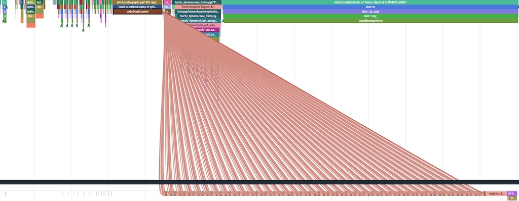
Trace Analysis: What Happens in 7ms
Chrome traces were exported and analyzed programmatically (30,783 GPU kernel events across 531ms). Here’s what a single decode step looks like:
[CUDA Graph: 36 layers, ~460 kernels replayed as one launch]
  ├── RMSNorm (2.5us) → QKV matmul (14us) → RMSNorm (3us) → RMSNorm (3us)
  ├── RoPE + KV store (2+2+2us) → Flash Attention (28us)
  ├── Output matmul (11us) → RMSNorm (2.5us) → Gate/Up matmul (40us)
  ├── SiluAndMul (3us) → Down matmul (26us)
  ├── ... (x36 layers)
  └── Final RMSNorm
[compute_logits: LM head matmul, 294us]
[Sampling: softmax + argmax + random, ~189us]
[~~~ CPU BUBBLE: 909us avg ~~~]  ← scheduler, postprocessing, next batch prep
[Next step...]
Decode steps are remarkably consistent: 7,095us median, varying only 6,918-7,637us. The first few steps are slightly slower (all 128 sequences active), and the last few slow down as batch sizes shrink to odd numbers that don’t align with graph capture sizes.
GPU Occupancy: 79.9%
The GPU is idle 20% of the time (107ms out of 531ms). Where do the gaps come from?
| Gap Source | Total Time | % of Gaps |
|---|---|---|
| Post-sampling CPU bubble | 57 ms | 53% |
| Sub-microsecond inter-kernel gaps | 13 ms | 12% |
| Other gaps | 37 ms | 35% |
The sampling bubble is the single biggest source of GPU idle time. After the sampling kernel finishes, the GPU waits ~900us for the CPU to: check for finished sequences, update token lists, run the scheduler, and prepare the next batch’s inputs. This happens 63 times (once per decode step), adding up to 57ms — 11% of total wall time.
CUDA Graph Efficiency in Decode
The CUDA graph captures the entire 36-layer model forward pass — all ~460 kernels per decode step are replayed as a single cudaGraphLaunch call (~400us CPU time). Without the graph, each of those ~460 tiny kernels (many under 5us) would need individual CPU dispatch at ~2-3us overhead each, adding ~1-1.4ms of pure launch overhead per step. The graph eliminates this entirely.
What remains outside the graph per step:
compute_logits— the LM head matmul (294us)- Sampling kernels (189us)
- CPU bubble (909us) — scheduler, postprocessing, next batch preparation
The CPU bubble is the clear remaining bottleneck. Overlapping it with GPU compute is tempting, but there’s a real data dependency: the next step’s input_ids are the sampled tokens from the current step. You can’t launch the next forward pass without knowing what was sampled. That said, the sampled tokens are already in GPU memory — keeping them there (device-to-device copy into the next graph’s input buffer, without a CPU round trip) and deferring EOS checking to run asynchronously could shrink the bubble. This is roughly what vLLM’s async output processing does, though the details are non-trivial.
What About Prefill?
Prefill does not use CUDA graphs. Each prefill step has a different sequence length, so the input shapes vary — violating CUDA graph’s fixed-shape requirement. CUDA-graphing prefill would require padding all prefills to a fixed maximum length and masking out the padding — the wasted compute on padding tokens often outweighs the launch overhead savings. Some engines (like TensorRT-LLM) do this for small prefills, but it’s a trade-off that depends on the input length distribution.
Key Takeaways
-
Read nano-vllm before reading vLLM. The ~1,200 lines cover every major concept in LLM inference: paged attention, continuous batching, prefix caching, CUDA graphs, tensor parallelism, and torch.compile. Once nano-vllm makes sense, vLLM’s architecture clicks.
-
Profiler overhead matters.
with_stack=Trueandprofile_memory=Trueadded 548% overhead. For timing-sensitive analysis, use minimal options and always compare against an unprofiled baseline. -
2NDis a good approximation for inference FLOPs at short context lengths. The gap from attention FLOPs is <1% for typical chat workloads. -
MFU is batch-size-dependent. 4.4% at batch=16 vs 23.7% at batch=128 on the same GPU. Small-batch decode is memory-bandwidth-bound, not compute-bound.
-
CUDA graphs eliminate kernel launch overhead for the model forward pass, but the CPU scheduling bubble between steps (~900us) becomes the next bottleneck.
-
Chrome traces reveal what summary tables hide. The gap analysis showed that 53% of GPU idle time comes from a single source — the post-sampling CPU bubble — which isn’t visible in kernel time tables at all.