Machine Learning for Relevance

15 Sep 2018

In this blog, we will look at several practical machine learning algorithms and their industrial appliations.

• SVM
• XGBoost
• Conditional Random Fields
• Neural Collaborative Filtering
• Yahoo! Learning to Rank
  • Metrics
• Google Ads CTR
• Bing Sponsored Search CTR
• Facebook Ads CTR
• Google Play Recommender: Wide and Deep
• Didi ETA: Wide, Deep and Recurrent
• Gmail Priority Inbox per user Model
• Facebook Recommender using Matrix Factorization
• Twitter Topic classification
• Google TFX Platform
• Fake News
• Position Bias
• Possible topics

SVM

“A Practical Guide to Support Vector Classification”. C.W. Hsu, C.C. Chang, C.J. Lin. 2003. “Support Vector Machines”. C.J. Lin, Machine Learning Summer School 2006.

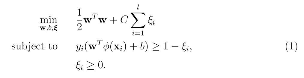
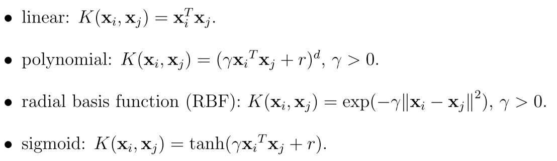
SVM is a large margin classififer, common kernels are The proposed procedure is:

• Transform data to the format of libSVM package. Use one-hot encoding for categorical features if it is not too large.
• Scaling feature to [-1, 1] or [0, 1]
• Consider RBF kernel. Kernel value is between 0 and 1. When num of features is large, try linear kernel.
• Use cross validation to find best $C$ and $\gamma$. Training accuracy does not count. Grid search with exponentially growing sequence, for example $C = 2^{-5}, 2^{-3}, \dots, 2^{15}, \gamma = 2^{-15}, 2^{-13}, \dots, 2^{3}$.
• Use best $C$ and $\gamma$ to train whole training set
• Test

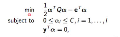
SVM dual problem, let $I$ be size of dataset Support vectors are the ones with $\alpha_i > 0$, prediction is

$$w = \sum_{i=1}^I \alpha_i y_i \phi(x_i) \\ w^T \phi(x) + b = \sum_{i=1}^I \alpha_i y_i K(x_i, x) + b$$

For kernel training, use dual formulation. But $Q$ is large, usually support vector is much smaller, use decomposition method similar to coordinate-wise minimization. Still does not scale to millions of data. Linear SVM scale well if num of features is small. There are more advanced approximation methods to scale SVM.

$$min_{w, b} 1/2 w^T w + C \sum_{i=1}^I max(0, 1 - y_i (w^T x_i + b))$$

For multi-class, train one-vs-all, then select one with largest response. When using one-vs-one, select the one with most wins.

XGBoost

Tianqi Chen and Carlos Guestrin. XGBoost: A Scalable Tree Boosting System. 2016.

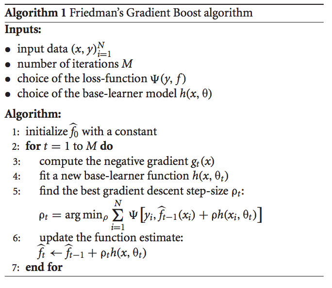
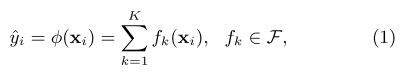
XGBoost is an efficient implementation based on Friedman’s graident boosting machines using regression trees. Define the following

$$\mathit{D} = \{(x_i, y_i)\} (\lvert \mathit{D} \rvert = n, x_i \in \mathit{R}^m, y_i \in \mathit{R}) \\ \mathit{F} = \{ f(x) = w_{q(x)}\} (q: \mathit{R}^m \rightarrow T, w \in \mathit{R}^T) \text{ regression trees} \\ I_j = \{i \mid q(x_i) = j\} \text{ be the instances landing on tree leave } j \\ g_i = \delta_{\hat{y}^{t-1}} l(y_i, \hat{y}^{t-1}) \\ h_i = \delta^2_{\hat{y}^{t-1}} l(y_i, \hat{y}^{t-1}) \\ \Omega(f) = \gamma T + 1/2 \lambda \lVert w \rVert^2$$

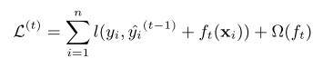
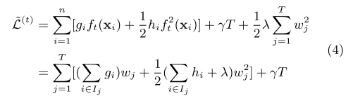
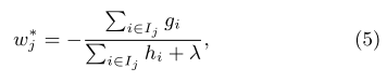
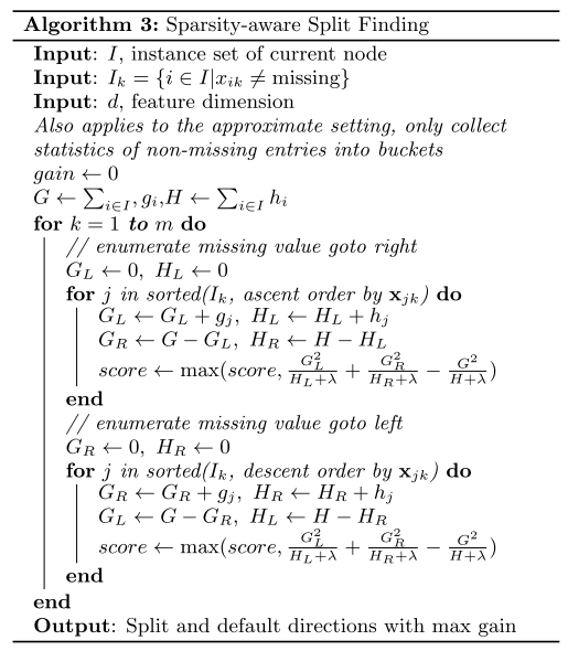
The loss function is equation 4, the optimal weights for given a tree is equation 5, the correponding loss is equation 6. 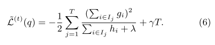The remaining issue is how to determine the structure of each tree. Equation 6 can be used to evaluate the reduction in loss function after spliting a tree node. The exact method will test all features and all value of each features. The approximate algorithm will split feature values into equal weighted percentile buckets. There is a streaming version called GK quantiles summary algorithm. This paper proposed a weighted version, where the weight is the $h_i$. We won’t go into details here though. Data is usually sparse, eg many zero values, the spliting algorithm compute the splits by assigning a default direction to missing feature values. For machine learning with large amount data, the input pipeline can be a bottleneck. Data is stored in compressed sorted blocks via compressed column (CSC) format, it can be on disk acorss multiple machines. This format support parallel split finding. Since only key is sorted, the cache access pattern for data is random, prefetching minibatch can help avoid cache miss.

Experiments shows XGBoost has exellent learning quality and works efficiently for single box, out-of-core and distributed settings. It is better to encode categorical features as one-hot, and let missing value be zero according to blog. It is also better not to encode user id directly for tree models, while logistic regression can handle them easiy as the following Bing paper suguests.

Conditional Random Fields

Charles Sutton, Andrew McCallum. An Introduction to Conditional Random Fields. 2010.

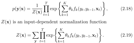
CRF is discrimitive model for sequence to sequence prediction, where output variable depends on each other. The paper coverage is large. Well known applications of CRF are POS tagging, named entity extraction (BIO), image segmentation etc. I also borrow from this note and this blog.

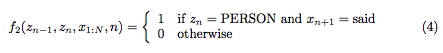
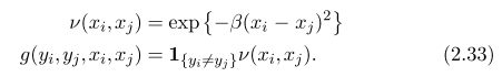
Here I only focus on linear chain CRF, whose inference and training method are very similar to HMMs and logistic regression. Engineers like CRF because it allows creative feature engineering, eg the following feature for NER should have a positive weight For image label/segmention, assigning different label to neibhours should be penalitied based on difference of image features

linear chain CRF inference is very similar to HMM, except transition and output factor is adjusted

• HMM forward algorithm
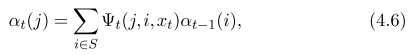
• HMM backward algorithm
• HMM transition marginal
• HMM evidence
• HMM viterbi Inference on general structured CRF can be done using belief propagation, or variational methods.

Training for linear chain CRF is using maximum likelihood, the graident of log likelihood with l2 regularization is 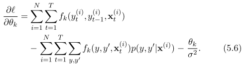This is the empirical count minus expected model count formula. To compute the expected count, transition marginal formula can be used. The log likelihood function is concave. This formula is amiable for SGD.

Neural Collaborative Filtering

He, X.; Liao, L.; Zhang, H.; Nie, L.; Hu, X. & Chua, T.-S. (2017), ‘Neural Collaborative Filtering’, CoRR abs/1708.05031.

Existing method is matrix factorization, Factorization machine is a generalization. For implicit feedback, data is 0 and 1, negative by sampling unobserved. Here we use logloss instead of squared loss.

Combine two models linear inner product matrix factorization (GMF, general here means the loss is logloss). Nonlinear embedding through MLP. Use Adam to train (per feature learning rate) separately then average before logloss and train together using SGD. MLP embedding size is 16, three layers of MLP reducing size from 32, 16 to 8.

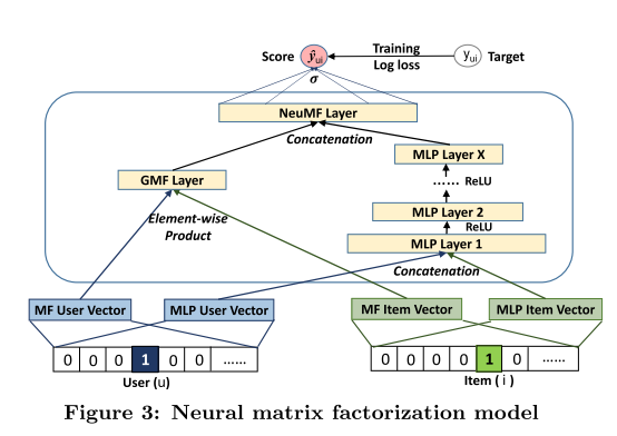
Evaluation metric is leave-one-out: for each user leave his latest interaction out, and rank it with 100 randomly selected unobserved items and evaluate NDCG@10. Compared with eALS, where weight is based on item popularity.

Yahoo! Learning to Rank

Ranking Relevance in Yahoo Search. Dawei Yin, Yuening Hu, Jiliang Tang, Tim Daly, Mianwei Zhou, Hua Ouyang, Jianhui Chen, Changsung Kang, Hongbo Deng, Chikashi Nobata, Jean-Marc Langlois, Yi Chang. Published 2016 in KDD

Many topics to improve relevance.

Three levels of ranking, shard light weight score for text matching, core ranking functions, blender contextual rerank.

• features: web graph, document, query, text matching (in various sections and anchor text), topical mathcing, click, time.
• core ranking (indexer): Ranking function is using logistic loss, which perfect and exellent are considered positive. This is good at removing less relevant urls. For ranking properly, scale the gradient. For real web search, >99% are bad urls. On this dataset, contrary to the public learning to rank, this works better than LambdaMart. LambdaMart directly optimize NDCG, although it is not differentiable. The trick is to use the weighted change of NDCG when swapping one URL with all other URL. The same method can be used to opimize many other ranking based metrics.
• contextual reranking (blender) just on 30 top urls. eg use core ranking ranks as features. did not talk about the actual model here.

Query rewriting by machine translation from query into document title, eg translate how much into price. Training data is the clicked query document pairs. Learn phrase-level translations. not sentence level. In decoding it has to evaluate breaking into phrases and alignment etc. The null-word alignment is large 0.9. To evaluate the candidates, use another scoring function. Features of the scoring function can be translation score and feature specific to search. eg the jaccard similarity of urls shared by the two queries in the query/doc click graph. Some kind of beam search on hmm. In blender, the documents are merged from the original and the rewritten query. 100 million query rewrite cache to reduce latency.

Compute semantic embedding for query and document through deep learning based on paper. Inputs are bag of words of query and clicked and nonclicked document. Convert to bag of trigram total 30k, severl layers with tanh activitation, get 128 dimension embedding vector. Loss is softmax of cosine(query, document) to predict click or not. Use 4 document per query, only 1 is clicked. Use softmax for pairwise training.

Only top queries has enough clicks. For other queries, use the following to compute similarity features for query and documents:

• bipartite query/document, propagate vocabulary back and forth. compute similarity of query/document over query vocabulary on runtime. Feature CS is the top one feature.
• machine translation, translate query into document title, then match with each docu title. Features from TLM are the 7th and 10th most important features.
• Deep semantic matching score using NN. Feature DSM is the eithth most important feature.

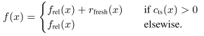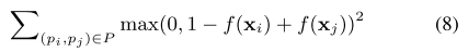
There are two classifiers to identify recency and location sensitive queries. For recency, adjust the DCG into recency-demoted relevance and tree additional trees to optimize for the delta. For location, add the correction terms Training uses a large margin objective for $P = \{ (p_i, p_j) \mid p_i \succ p_j \}$

Metrics

dcg: $DCG_N = \sum_{i=1}^N \frac{2^{g_i} - 1}{\log_2(i+1)}$. An implementation. $g_i$ are the true score, the list is first ranked using predicted score.

Averge precision is the area under precision recall curve. The AP@K metric is considering ranked list up to position k. It can be calculated as $\sum_{k=1:K} (\text{precision at }k * \text{ change in recall at } k)$.

ROC curve is true positive rate (TP / positive) vs false positive rate (FP / negative). AUC is its area.

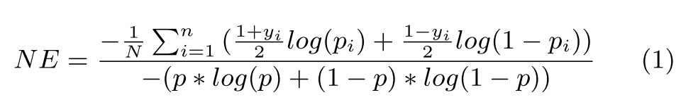
Normalized Entropy: average cross entropy normalized by cross entropy using avergage prediction. Assume y is either 1 or -1

Google Ads CTR

H. B. McMahan, G. Holt, D. Sculley, M. Young, D. Ebner, J. Grady, L. Nie, T. Phillips, E. Davydov, D. Golovin, S. Chikkerur, D. Liu, M. Wattenberg, A. M. Hrafnkelsson, T. Boulos, and J. Kubica. Ad click prediction: a view from the trenches. In KDD, 2013.

Billions of features, half of them only appear once in training data. I guess the features could be individual words and their combinations, instead of a text matching score as in search. Training is streaming online.

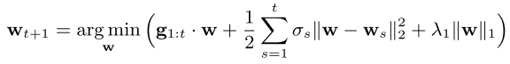
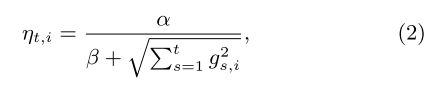
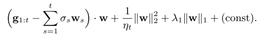
The CTR model is based on logistc regression The online learning algorithm is called FTRL, which choose parameter at time $t$ to reduce the regret so far with a regularization. Instead of using same learning rate $\eta_t = \frac{1}{\sqrt{t}}$, due to sparsity, more active parameter should have a smaller learning rate The full FTRL learning algorithm is. $n_i$ is the sum of square of derivative, $z_i$ is $(g_{1:t} - \sum_{s =1}^t \sigma_s w_s)$, $\lambda_2$ is an additional L2 penalty besides L1. The algorithm stored $z_i$ instead of $w_i$. 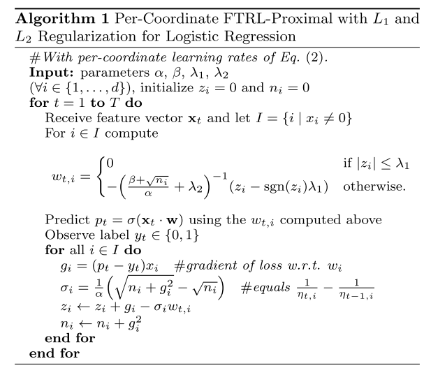The truncated gradient only does $l_1$ update every $k$ iterations to avoid truncate a new feature as in blog. Not sure how FTRL deals with new feature truncation. In experiments, FTRL is better than RDA in sparsity and AUC.

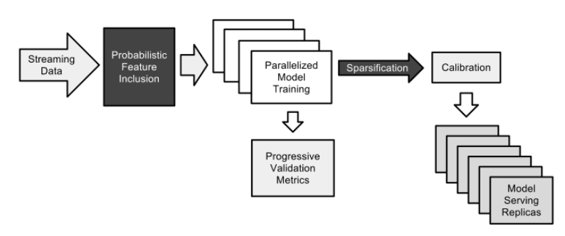
Practical issues:

• Reduce num of features by probabilistic feature inclusion. Hashing does not work.
• Clip $w$ with $[-4, 4)$, then use 13 bit fixed point format.
• Sharing feature weight across different models.
• Subsample negative data, wegith each negative by 1 over sample rate.
• Absolute metric value are often misleading. logloss when ctr is close to 50% is mucher higher even if prediction is perfect than when ctr is close to 2%. Look at relative changes compared with a baseline. Eg the normalized entropy metric.
• Compare model across many dimensions through visualization.
• Confidence of a prediction measured by changes in prediction from parameter update?
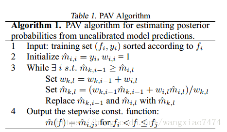
• Isotonic regression for calibration. Platt’s scaling is training a one dimension logistic regression.
• Metadata for thousands of signals (generate features), eg versioning
• Unsuccessful exepriments: dropouts, feature hashing, feature bagging, feature vector normalization.

Bing Sponsored Search CTR

Thore Graepel, Joaquin Quiñonero Candela, Thomas Borchert, Ralf Herbrich. Web-Scale Bayesian Click-Through Rate Prediction for Sponsored Search Advertising in Microsoft’s Bing Search Engine. In ICML, pages 13–20, 2010.

Generalized Second Price (GSP) auction: advertiser provide bids for keywords. Order by $p_i b_i$, payment of clicked ads at position $i$ is $c_i = b_{i+1} p_{i+1} / p_i$ to avoid dynamic bidding behavior.

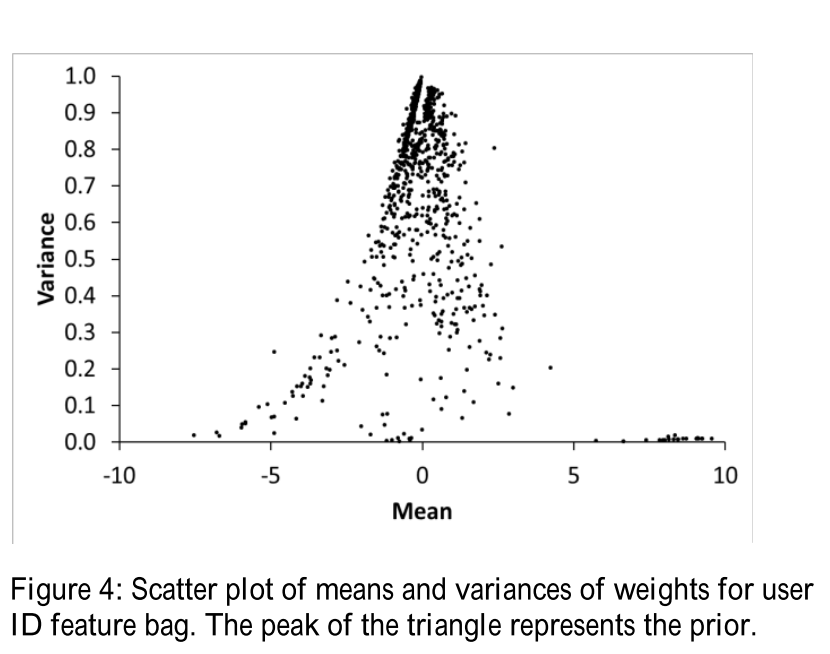
Adpredictor is an online Baysian probit regression method. 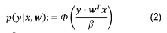Models the weight of each feature with a gaussian distribution. The prediction result for each sample is also a gaussian distribution. $i$ is feature index, $M_i$ is num of values of feature $i$. $x = (x_i^T, \dots, x_N^T)^T$, each $x_i$ is a one hot vector. $y \in \{ -1, 1\}$ as non-lock, and click. 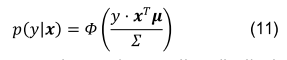The posterior of each $w_{ij}$ is a guassian with 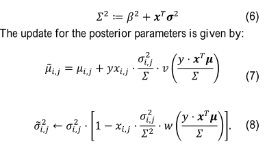Positive example makes mean increase, negative example reduce the mean. The amount of update is determined by normalized variance and how bad the current prediction is (controlled by $v$ and $w$). The prediction is One derivation of the message passing can be found in dongguo’s blog and another blog.

Practical issues:

• To avoid shrinking parameter variance to zero, previous likelihood is decayed, so inactive features will slows reset to prior.
• Model is not sparse, a feature is reset to prior based on KL divergence.
• Message passing support parallel training across machines, the master weight variable accumulae the results from all compute nodes. This is simialr to a parameter server.
• Model affects future training data. The logloss will increase with time even if model does a good job.
• Exploration by sample $w$.
• Features: ads, query and context. binary feature and billion-valued feature such as user id.

Facebook Ads CTR

Xinran He, Junfeng Pan, Ou Jin, Tianbing Xu, Bo Liu, Tao Xu, Yanxin Shi, Antoine Atallah, Stuart Bowers, Joaquin Quiñonero Candela. Practical Lessons from Predicting Clicks on Ads at Facebook, International Workshop on Data Mining for Online Advertising (ADKDD). 2014.

Use 500 GBM L2-TreeBoost trees to learning features, use online SGD logistic regression with per coordindate learning rate to train. Do many pushes to ranker daily to keep model fresh.

Details:

• Advertiser bids on demograph and interest targeting, not keywords.
• Feature engineering: bin continuous features, cross features. A tree become a categorical feature with each leaf as a category.
• Use normalized entropy as metric, where base learner is the avg CTR.
• Online SGD logistic regression with FTRL per coordindate learning rate is as good as Bing Bayesian Online Probit Regression (BOPR). Paper also tested constant learning rate, per weight learning rate etc. LR only requires half the memory and computation than BOPR.
• For streaming online training, requires a online joiner to have a window to wait for click joint. The trainer periodically emit new model to ranker.
• Detect anomalies eg the click stream could stop.
• Boosted tree training may take more than 1 day, only update weekly.
• Measure feature importance based on reduction in loss when spliting the variable in trees. Top 10 features accounts for half of the total importance.
• Historical features (past performance of an ad or user) is slightly more important than contextual infor (eg, time of day, page user is visiting). But contextual feature is important for cold start problem.
• Each day has about 10 billion ad impressions, use 10% of data to train is good enough. Downsample negative to 0.025 is best, calibration is just multiple predicted ctr by a factor to get back the avg ctr. If $w$ is the rate of negative subsample, then corrected prediction is $\frac{p}{p + (1-p)/w}$.

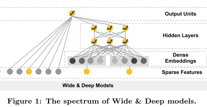
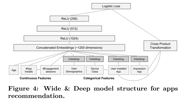
Google Play Recommender: Wide and Deep

Wide & Deep Learning for Recommender Systems. Heng-Tze Cheng, Levent Koc, Jeremiah Harmsen, Tal Shaked, Tushar Chandra, Hrishi Aradhye, Glen Anderson, Greg Corrado, Wei Chai, Mustafa Ispir, Rohan Anil, Zakaria Haque, Lichan Hong, Vihan Jain, Xiaobing Liu, Hemal Shah. arXiv:1606.07792 (2016)

Recommendation is similar to ranking problem. Logistic regression is simple, scalable and interpretable. Use sparse feature crossing to memorize pattern, eg AND(user_installed_app=netfix, impression_app=pandora). Generalization using embeddings can provide interactions unseen, but it may overgeneralize for sparse data. Use simple rule sto restrict candidate before passing to a ranking model. Final model is joint trained, instead of ensemble. Use FTRL with L1 for wide part and AdaGrad for deep part.

Features, map continous feature to quantiles. The wide component consists of the cross-product transformation of user installed apps and impression apps. 50 billion training examples, where label 1 if recommended app is installed.

Wide and deep is also applied to censor to predict income. The wide and deep parts pretty much work on same set of features, except the explicit crossing in wide part.

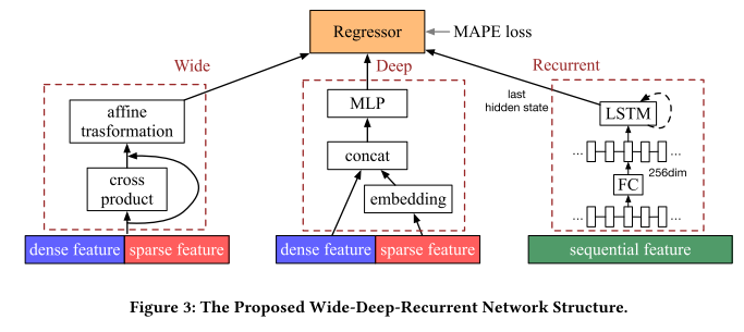
Didi ETA: Wide, Deep and Recurrent

Learning to Estimate the Travel Time. ZhengWang, Kun Fu, Jieping Ye. KDD 2018.

Traditionally overall travel time of a given route is formulated as the summation of the travel time through each road segment and the delay time at each intersection. Here formula as a regression problem.

Feature:

• road: obtain road segments, extract info about each segment, eg length, width, num of lanes, POIs.
• temporal: rush hour indicator
• traffic: real time estimated speed
• driver info: style, vehicle
• whether, traffic restriction

Off the shelf models are GBDT, FM (feture interaction through embedding crossproduct). Combine three models wide, deep, recurrent. Wide is cross product dense feature then logistic regression with FTRL, deep part embeds sparse feature (user id), recurrent handls the variable length road segment features, the other two model use a statistical summary of segments to have fixed length features. Recurrent model use LSTM. When data is large, deeper model has more advantage, shallow model is a special case of deeper ones. Metric is Mean Absolute Percentage Error (MAPE), worse at roush hour. GBDT 23.6%, FM has 21.4%, WDR has 20.8%.

Gmail Priority Inbox per user Model

Hundreds of features: social, content (headers and terms), thread, email filter label. Continuous features are converted to binary by ID3 splitting using information gain (reduction in entropy). Features are calculated in ranking, and stored for training. Model predicts $p = Pr(a \in A, t\in (T_{min}, T_{max}) \mid f, s)$, $T_{min}$ is less than 24 hours, $T_{max}$ is days. $s$ indicates user has opportunity to see the mail.

Each message update global and per user model. Per user model include additional per user features. Use passive-aggressive updates [2]. Per user threshold for importance or not, some user prefers to see more email. Realtime join is by bigtable directly. training by batching users that share a prefix, use off-peak machines, a lot of saving than true online learning. Use user manual marked emails for evaluation. Use bigtable to estimate the last time a user was active in Gmail.

Facebook Recommender using Matrix Factorization

https://code.fb.com/core-data/recommending-items-to-more-than-a-billion-people/

Recommend facebook pages and groups. use giraph, rotational hybrid apporach by worker send each other message to reduce shuffle size.

top-k item recommenation, hold item vectors using ball tree, use upper bound to prune. Another way is to form k-means clustering of item feature vectors, and restrict recommendation to nearby clusters. Seems Faiss can also be used as this is nearest neighbor search.

Block ALS in spark. Only send once per block, ratings are stored twice. Giraph is 10x faster, can handle 100 billion ratings.

Explicit negative feedback is not easy to get, use weighted random sampling for negatives. Also use the implicit formulation.

The implicit CF converts into weighted ALS.

Twitter Topic classification

Large-Scale High-Precision Topic Modeling on Twitter. Shuang Yang, Alek Kolcz, Andy Schlaikjer, Pankaj Gupta. KDD 2014.

TAXONOMY 300 topics from ODP and freebase, also map LDA clusters to topics.

Tweet text classification using unlabeled tweets:

• First filter by Chatter classifier.
• human annotation is costly, hard for 300 topics and niche topics, only used for evaluation. Confirmation labeling is easier. Use probe task to weed labelers.
• Positive tweet: Use priors from user rules, entity rules (nba), url rules (urls with nba) to filter. co-training two classifiers for tweets with URLs: URL classifier and tweet classifiers. Did not use active learning, still need millions of tweets given sparsity of a tweet.
• Negative tweet: random sample is not accurate. PUlearning [12] Rocchio classifier [20].
• Features: tweet is short, use byte 4grams hased to 1million. For webpage, use hashed unigram with log(1+tf) then normalized by l1 norm. The normalization improves quality for long web documents.
• Use LR one-vs-all, considering the taxonomy hierarchy, eg negatives should have include postives for its chidren. The cost of errors is different based on distance on the tree. Use parent weights to regularize children weights.
• Select threshold to achieve a precision target. Stratefied sampling by breaking predicted probability into buckets. Confirmation labeling to estimate precision of each bucket. Weight precision by size of each bucket to achieve desired precision.
• UI to show tags for feedback, corrective learning [25, 23] to fix mistakes.
• Fine tune with high quality data by adding regularization to weights learning from large scale noise data. Shrinkage to prior can be used for when new data is coming in batches. ADMM for distributed training.

User Interest:

• Collect user produced and consumed tweet topics, do a tf-idf weighting, then softmax. Decay to model interest shift.
• List mapped to topics, users there maps to knownfor, followers become interested in.

Hashtag to topics:

• A linear model to predict topic based on correlation of hashtag and topics.

A tweet has text, tweeter, engager, hashtag, url, each provide a predict over topics. Ensemble them by learning a weighted combination. The weights are trained using adaboost algorithm.

Google TFX Platform

TFX: A TensorFlow-Based Production-Scale Machine Learning Platform. 2018.

machine learning platform (as a service)

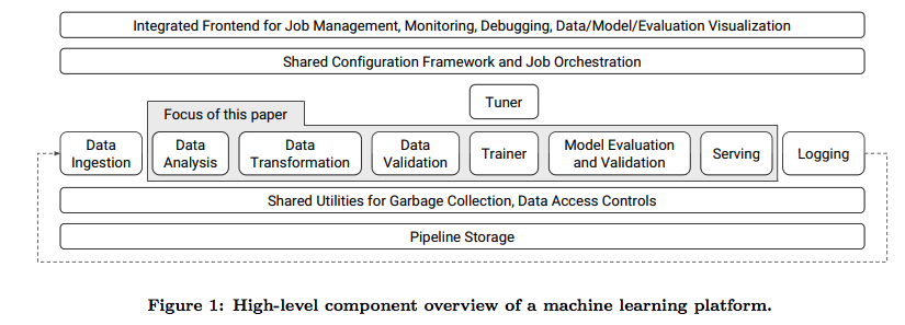
1. support many learning tasks. using tensorflow
2. continuous training/serving. not just workflow jobs. data visitation
3. UI for minotoring and analyze
4. reliable and scalable. validate data, model and serving. similar to Apache Beam.

data analysis, transformation and validation.

• anomalies, errors, alert user
• descriptive statistics for data and features
• assign id to sparse feature values.
• user provide schema for expected feature properties. filter bad example.

continuous training with warm start

• Can restore selected features.
• New data arrive in batches.
• using Estimator and FeatureColumns for higher abstraction. eg tf.feature_column.categorical_column_with_vocabulary_list, tf.estimator.DNNRegressor.

model eval and valuation

• safe to serve: trained in new version but serving is on old version.
• offline evaluation on AUC or approximate business metrics before live A/B testing
• canary process
• slicing

tensorflow serving:

• use separate threadpool for loading
• tf.example protocol buf for NN, for non NN, a special proto for data.

Fake News

Fake News Detection on Social Media: A Data Mining Perspective. KDD 2017.

new features: publisher, content (linguistic features), engagements (user average followers, post, time). propagation features.

Position Bias

Unbiased Learning-to-Rank with Biased Feedback Thorsten Joachims. Thorsten Joachims, Adith Swaminathan, Tobias Schnabel. arXiv:1608.04468v1

Empirical risk minimization with expert judement: The loss of a ranking function is the averge negative DCG over training data.

The probability $Q(o_i(y) = 1 \midx_i, \bar{y}_i, r_i)$ of observing the relevance ri(y) of result y for query xi is the propensity of the observation.

Possible topics

• AirBnB Search Personalization
• Machine Translation
• Kaggle
  • https://medium.com/unstructured/how-feature-engineering-can-help-you-do-well-in-a-kaggle-competition-part-i-9cc9a883514d
• position bias
• query rewrite: based on thesaurus build by word coourrence, query log mining, spell correction.
• Machine Learning Systems
  • feature mangement: database
  • hyper-parameter tuning
  • Live model performance monitoring, alert: business metrics and model specific metrics
• AB testing