Several Object Detection Papers
07 Aug 2017This blog is about object detection deep learning papers. Note that Ross Girshick is on the authors list for all of them!
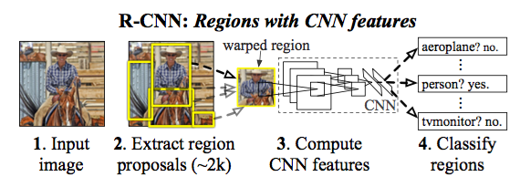
R-CNN
R. Girshick, J. Donahue, T. Darrell, and J. Malik. Rich fea- ture hierarchies for accurate object detection and semantic segmentation. In CVPR, 2014.
selective search for region proposal, AlexNet to compute region image features 4096 vector, then binary SVM classify label and linear regression to correct bounding box proposal. NMS to remove overlapping. 53.3% mAP on VOC 2012.
Training procedures:
- Pretraining on imagenet.
- Use proposed region to finetune AlexNet on 21 classes (20 VOC classes plus background), each minibatch has 32 positive windows and 96 background windows. Positive and negative window is determined by IoU 0.5.
- Train one SVM per class using extract last fully connected layer 4096 features. Positive is ground truth bounding boxes, negative examples are regions with IoU < 0.3, use hard negative mining method.
- Train linear regression on pool5 features to correct bounding box.
Visualize last convoultion layer $6x6x256$, by running over heldout images and collect receptive field regions that has large activations on each of the $256$ features.
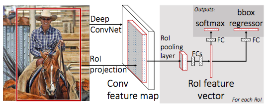
Fast R-CNN
R. Girshick. Fast R-CNN. In ICCV, 2015.
68% mAP on VOC 2012, prediction is 300ms per image excluding region proposal time.
R-CNN is slow because it performs a convnet forward pass for each proposal. In Fast R-CNN, one forward pass can score all proposals. For VGG16, the last max pooling layer is replaced with RoI pooling, which always generate a 7x7 sized output for any sized proposal. The last fully connected layer and softmax is replaced with two similarly structured branches, one for object prediction (21 for VOC), and one for bbox regression for each object class (4*20 for VOC). With 2000 proposals per image, after RoI pooling layer, 1 image become 2000 batched input to the rest of the fully connected layers.
The whole network is trained end2end by sampling 2 images and 69 proposals per minibatch. The network is pretrained from ImageNet, the fully connected layers in the two branches are randomly initialized. The learning rate for the two is 1 for weight 2 for bias, rest of the weights are 0.001 for fine tunning.
Some findings from experiments:
- truncated SVD (two layers $\sum_t V^T$, then $\sum_t U$)for fully connected layer make model smaller ($u v$ vs $t*(u+v)$), 45% faster with 0.3% drop in mAP.
- If only fine tune $\geq fc6$, mAP drop 6%.
- Training and predicting pyramid give $\leq 1%$ mAP.
- end2end softmax is slightly better than post-hoc SVM.
- More region proposal for retraining may not improve mAP.
Faster R-CNN
S. Ren, K. He, R. Girshick, and J. Sun. Faster R-CNN: To- wards real-time object detection with region proposal net- works. In NIPS, 2015.
200ms per image using 300 proposals. winner of ILSVRC 2015 object detection. 1st place of COCO 2015 object detection competition.
Use region proposal network to replace selective search, share same base network with Fast-RCNN.
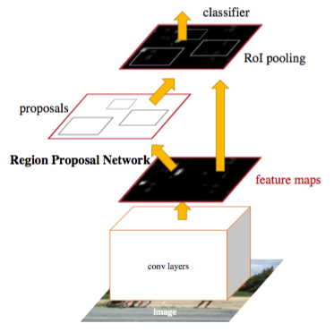
RPN is a sliding-window (implmented as convolution) class-agnostic object detector, use 3x3 window, each windows has 9 anchors (3 scale 3 aspect ratio), so we use a fixed window to predict boxes of various sizes. The $3x3x512$ is projected to $512$ first. The total parameters for the softmax layer (1x1 conv) is $512 x (4+2)*9$. The loss function for bound box is in the view of an anchor by transforming both ground truth and predict in terms of the offset to each anchor. Negative anchors are downsample to have same num as positive per image. Postive has $> 0.7$ IoU, negative has $<0.3$ IoU, rest are ignored. RPN proposals may highly overlap, after NMS the top 2000 are passed to Fast R-CNN.
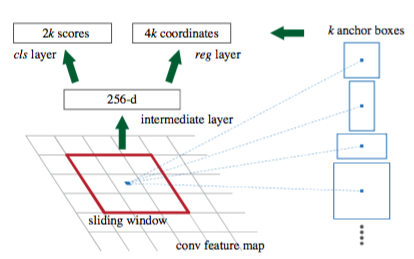 In experiment use 600 pixel input (network is FCN, it is able to accept any sized, not too small, input), 228 pixels receptive field for the 3x3 RPN window. For $1000 \times 600$ input, total about $60 \times 40 \times 9$ anchors.
Achors sizes: $128^2, 256^2, 512^2$, so allow predictions that are larger than the underlying receptive field.
In experiment use 600 pixel input (network is FCN, it is able to accept any sized, not too small, input), 228 pixels receptive field for the 3x3 RPN window. For $1000 \times 600$ input, total about $60 \times 40 \times 9$ anchors.
Achors sizes: $128^2, 256^2, 512^2$, so allow predictions that are larger than the underlying receptive field.
Training:
- alternating training RPN and Fast-RCNN to share the same base network, initialize first RPN from imagenet pretrained weights.
- Need to ignore cross boundary anchors only in training, otherwise they introduce large, difficult to correct error terms. training will diverge.
FPN
T.-Y. Lin, P. Dollár, R. Girshick, K. He, B. Hariharan, and S. Belongie. Feature pyramid networks for object detection. InCVPR, 2017.
FPN is used by both Mask R-CNN and RetinaNet. It is an efficient way to simulate image pyramid. For base network ResNet, stage $C_2, C_3, C_4, C_5$, add the following top down stucture, after merge with lateral connection, add a 3x3 convolution to reduce aliasing in upsampling. This becomes $P_2, P_3, P_4, P_5$. All of them has channel depth 256 to share network heads weights etc across layers. Upsampling is by use nearest neighbor upsamling.
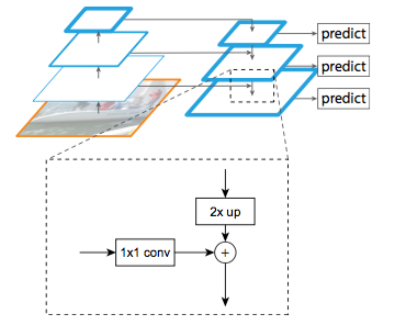
For RPN network, we add the network head as in the Fast R-CNN section to each layer, but no need to use multiscales, instead use $32^2, 64^2, 128^2, 256^2, 512^2$ anchor size and the 3 aspect ratios. So total 15 types of anchors over the pyramid. All network head share same parameter across different layers (also tries using different parameters, similar accuracy). In the original RPN, parameters are not shared across scale $512 \times (4+2) \times 9$. Now it is either $512 \times (4+2) \times 3$ or $512 \times (4+2)$ depending on whether parameter is shared across aspect ratios. This becomes a pyramid RPN.
For Fast R-CNN, we attach the same detection Head to all layers with shared parameters. The RoI detected by RPN may not be classified in the same layer through, the formula is $k = floor(4 + \log_2(\sqrt{w h} / 224))$.
On Coco, 36.2% test-dev mAP, 35.8% test-std. Also try segmentation, on each level, output 14x14 mask and object scores (guess as a softmax across classes per pixel).
Mask R-CNN
K. He, G. Gkioxari, P. Dollár, and R. Girshick. Mask R-CNN. In ICCV, 2017.
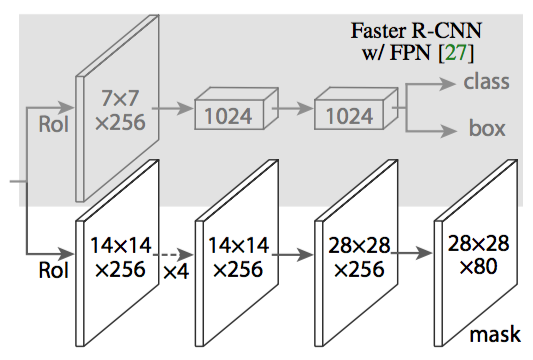
Based on Faster R-CNN, added a mask predicition branch, which are serveral layers of conv and deconvdeconvolution to upsample. The m×m floating-number mask output is then resized to the RoI size, and binarized at a threshold of 0.5. The mask is binary, the predicted class of the ROI is used to pick the right mask.
Good results on detection, instance segmenation, human pose estimation, two reasons for success
- RoIAlign is similar to RoIPool, except quantization in division is replaced by interpolation. For example when transforming RoI coordindates to feature map location based on stride, the extracted feature is interpolated by neighbors. Similarly when dividing feature map into 7x7 grid.
- Existing FCN usually perform per-pixel multi-class softmax classification. Mask R-CNN’s mask is binary mask per class, no competition between classes.
Experiments:
- Instance segmenation on Coco, ResNeXt-101-FPN get 37.1%. Use ResNet-101-C4 as backbone gets 32.7%.
- Multinomial mask reduce mAP 5.5%.
- One mask for all classes is nearly efective!
- RoIPool reduce mAP by 3%.
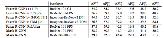
- Coco object detection mAP 39.8%.
- For human pose, each keypoint is a seperate class. Mask loss for each keypoint, a $m^2$ way softmax loss. Between keypoint classes, still independent. As data is small, use muliscale training as augumentation. Added two bilinear upscaling to get output $56 \times 56$ to improve keypoint localication accuracy.
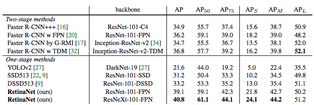
The result comparsion on Coco test-dev set.
Retinanet
T-Y Lin, P Goyal, R Girshick, K He, P Dollár. Focal Loss for Dense Object Detection. IEEE International Conference on Computer Vision (ICCV), 2017.
Paper proposes focal loss to improve one pass object detection. class imbalance is the culpit for low quality of one pass, because cross entropy loss is still high for easy example, given large num of them (for example many background patches), their sum will overshadow hard examples. focal loss multiplies cross entropy loss by $(1-p)^2$ when $y=1$ and $p^2$ when $y=0$, so easy examples are highly discounted. It uses all 100k backgroudn patches in training. It is also better than online hard-example mining. It initialize the sigmoid bias to be $\log(0.01/(1-0.01))$ to bias initial prediction to be background to avoid accumulating large losses initially.
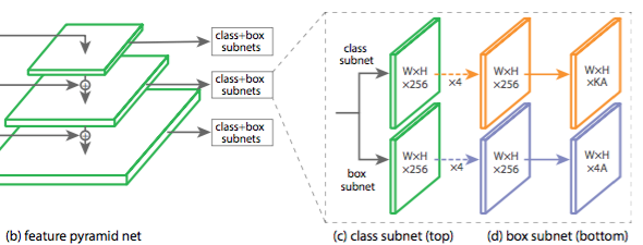
Retinanet is similar to the RPN network with FPN as base. With the following differences
- Add detection head to layers $P_3, P_4, P_5, P_6, P_7$. Here $P_6$ and $P_7$ are added by 3x3 stride 2 conv ontop of $P_5$ to detect larger objects. Anchor size is from $32^2$ to $512^2$. Besides the 3 aspect ratio, here each level has 3 sizes by multiple size of the level with $1, 2^{1/3}, 2^{2/3}$, so total $5 \times 3 \times 3$ anchors types. $A=9$.
- The classification and regress head does not share parameters, each share parameters across different levels by themself.
- The bbox regression is class agnostic.
- The class regression has $K$ classes.
Experiment:
- The bias initialization is import to converge.
- Focal loss gives 3.8% mAP over cross entropy loss (all 100k anchors using cross entropy loss work?).
- Focal loss improves 3.2% mAP over hard negative mining.
The result comparsion on Coco test-dev set.