Multiple View Geometry in Computer Vision
07 Dec 2017This blog is about Multiple View Geometry in Computer Vision by Richard Hartley and Andrew Zisserman. I will mainly take some notes about the gold standard algorithms in this book. All figures are blatantly copied from the book.
- 3D Space
- 2D homography
- Camera models
- Compute Camera Matrix P
- Single View
- Epipolar Geometry
- Computing Fundamental Matrix
- 3D reconstruction
- N-View
3D Space
Concepts:
- Plane is a 3 vector. 3 point define a plane, 3 planes define a point.
- Quadrics is a surface x^TQx = 0, Q is 4x4. its 2d counter part is conic.
- plane at infinity $\pi_\infty = (0, 0, 0, 1)^T$
- abosulte conic $\Omega_\infty$ is conic at infinity, $x_1^2 + x_2^2 + x_3^2 = 0$ and $x_4 = 0$
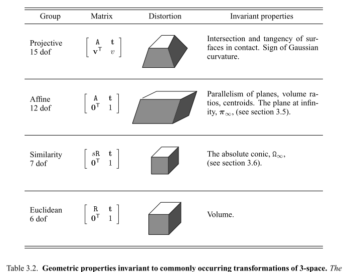
3D transoforms
2D homography
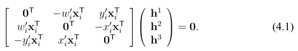
A plane in two views are related by a homography $H_{3x3}$. Two views if camera is only rotated about its center also has a homography. Given $x_i$ and $x_i^{\prime}$ are 2D correpondence point, use homogenous coordindates. From $x_i^{\prime} = \eta_i H x_i$, thus $x_i^{\prime} \times H x_i = 0$. let $\textbf{x}^{\prime} = [x_i^{\prime}, y_i^{\prime}, w_i^{\prime}]$, $h$ is the ith row of $h$. 4 points give 8 constraints $Ah = 0$, $A$ is $2nx9$. Let $A = UDV^T$, then $h$ is the last column of $V$. This is the Direct Linear Transform (DLT) algorithm (Algorithm 4.1 on page 91).
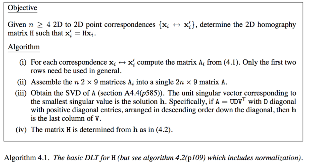 An improved algorithm is Algorithm 4.2 on page 109, it does prenormalization before calling Algorithm 4.1, so that the mean of $x$ are (0, 0) and average distance to origin is $\sqrt{2}$.
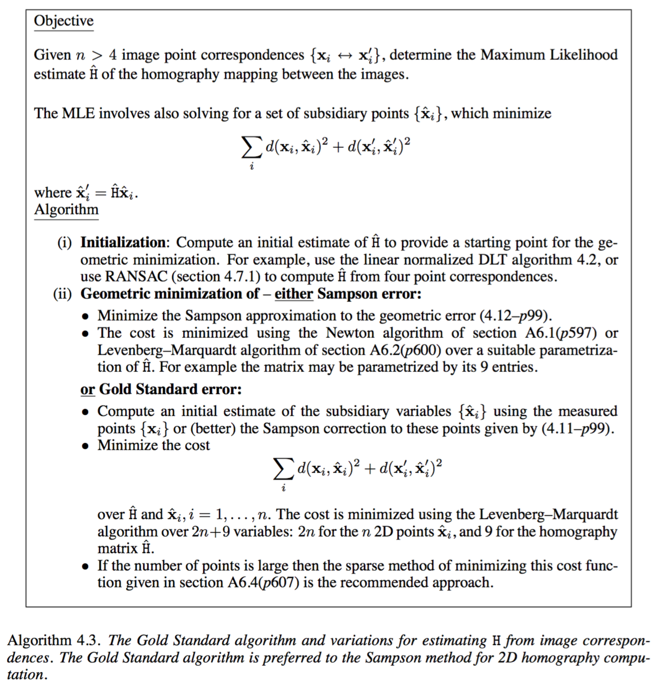
Given $H$, the projection of $x$ is $\hat{x}_i^{\prime} = Hx$, for $x^{\prime}$, its projection is $\hat{x}_i = H^{-1} x^{\prime}$. Use optimization to iteratively reduce reprojection error. This is the gold standard Algorithm 4.3 on page 114 for estimating H from image correspondences.
RANSAC randomly selects random candidate and measure num of inliners.
- Threshold: sum of squares of distance is a $\xi_m^2$ distribution.
- samples: $(1-w^s)^N = 1 - p$, so $w$ is inlier probability, $s$ is num of points, $N$ is num of selections, $p$ is confidence. When $w$ is unknown, can estimated it from current model.
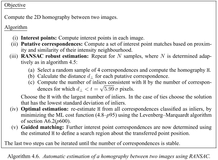
Homography using RANSAC Algorithm 4.6 on page 123.
Camera models
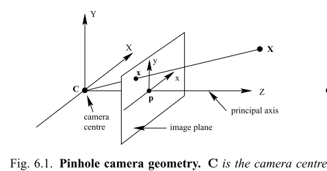
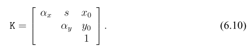
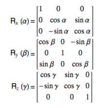
 Image point $x = P X$, $K$ is 3x3 upper-triangular matrix, $\alpha_x, \alpha_y$ is the focal length in pixels. $R$ is a 3x3 rotation matrix whose columns are the directions of the world axes in the camera’s reference frame. The vector $\tilde{C}$ is the camera center in world coordinates; the vector $t = -R\tilde{C}$ gives the position of the world origin in camera coordinates according to this blog. Rotation can be decomposed into rotation along x, y and z axes
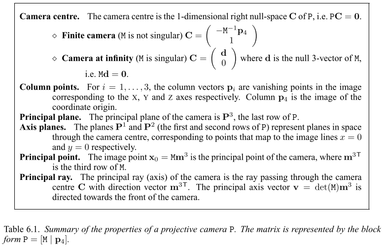 Recover intrinsic and extrinsic parameter from $P=[M \mid p_4]$, so $\tilde{C} = -M^{-1}p_4$. $K$ and $R$ can be separated by RQ-decomposition of $M$.
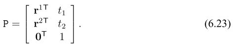
Cameras at infinity is affine camera, with last row of $P$ is (0, 0, 0, 1).
- Orthographic projection map (X,Y,Z,1)^T to (X, Y,1)^T.
- Weak perspecitive projection, is scaled orthographic projection, where $\alpha_x$ and $\alpha_y$ not equal.
Compute Camera Matrix P
P is $3x4$, similar to the 2d homograph derivation, because $x = PX$, we will have the following constraint
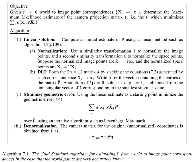
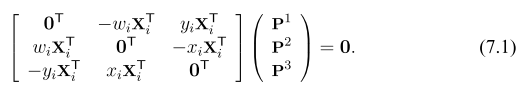 Similarly to solve $P$ with at least 6 points, this is the Algorithm 7.1 gold standard algorithm to estimate P, this is implemented in the popular camera calibration code in opencv with calibration grid. In fact, it also considers radial distortions.
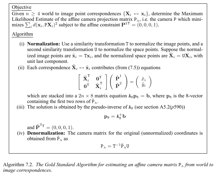
For affine cameras, we only need to estimate the first two rows, this results in the following Algorithm 7.2.
Single View
Vanishing point: a line in world $X(\lambda) = A + \lambda D$, D = (d^T, 0)^T. The vanishing point is the ray parallel to world line from camera center intersection with image plane, ie $Kd$. Two parallel world lines intersect at vanishing point.
Vanishing line: Intersection of image plane by a plane going through camera center parallel to the plane. $l = K^{-T} n$. Or connecting two vanishing points on the plane. Three equally spaced parallel lines can determine the vanishing line.
Algorithm 8.1 can compute ratio of two scene lines perpendicular to the ground plane.
Epipolar Geometry
In two views, a point in one view define a epipolar line in the other view on which the corresponding point lies, main concepts:
- epipole is the intersection of image plane by the line (baseline) joining the camera centers.
- All epipolar line intersect at the epipole.
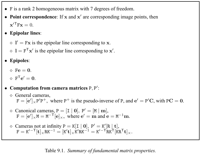
- Fundamental matrix $F$ is $3x3$, rank 2, corresponding image points $x’^T F x = 0$
- $P$ and $P^\prime$ may be computed from $F$ up to a projective ambiguity of 3-space, can be chosen as $P = [I \mid 0]$ and $P^\prime = [[e^\prime]_x F \mid e^\prime]$.
- For image point $x$, normalized coordindates of it $\hat{x} = K^{-1} x$
- Essential matrix $E$, two corresponding normalized coordindates has $\hat{x}’ E \hat{x} = 0$.
- $E = K’^T F K$
- $E$ is a essential matrix iff two of its singular values are equal, the third is zero.
- If $E = U diag(1, 1, 0) V^T$, first camera $P = [I \mid 0]$, there are four choices for the second matrix $P’$ $P’ = [U W V^T \mid \pm u_3]$ or $[U W^T V^T \mid \pm u_3]$
- If camera is affine, the first 2x2 of the fundamental matrix is 0, only need at least 4 point to compute $F$.
Properties of Fundamental matrix.
If $a=(x, y, z)^T$ then \([a]x = \begin{pmatrix} 0 & -z & y \\ z & 0 & -x \\ y & x & 0 \end{pmatrix}\)
Computing Fundamental Matrix
$f$ is the 9 vector from $F$ in row-major order, $x’Fx=0$ become
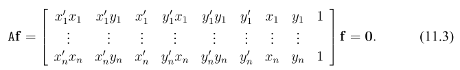
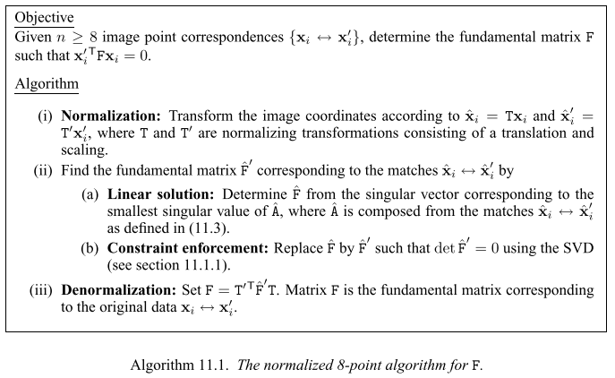 The trick is to replace $F = UDV^T$ by $F’ = U diag(r,s,0)V^T$.
The gold standard algorithm to compute fundamental matrix
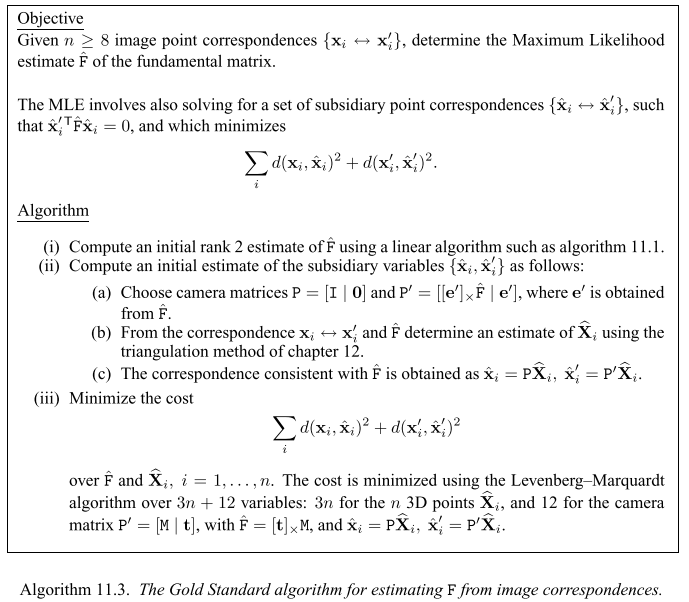
Image Rectification
Identify correspondences $x_i \leftrightarrow x’_i$, compute $F, e, e’$. Compute $H’$ maps $e’$ to $(1, 0, 0)^T$, compute the matching $H$ that minimizes $\sum_i d(Hx_i, H’ x’_i)$. The rectified images are remapped from $H$ transformation for $I$ and $H’$ transformation fro $I’$. An implementation is from cs231a.
3D reconstruction
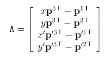
Given $x = P X$ and $x’ = P’ X$, again using the DLT method, $x \times (P X) = 0$, assuming the last component of $x$ is 1. Doing the same for $x’$, take two equations from the two and combine to become
$A X = 0$, solving use the SVD method to get the 3d point $X$.
 The actual optimal reconstruction algorithm 12.1 tries to minize the distance of $x$ and $x’$ to the epipolar line. It is much more involved than DLT though.
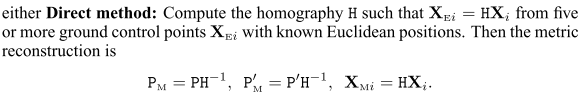
Metric reconstruction using direct method
N-View
Given the set of image coordindates $x_j^i$ find the camera matrices $P^i$ and the points $X_j$ such that
\(\min\limits_{\hat{P}^i, \hat{X}_j} \sum\limits_{i,j}d(\hat{P}^i \hat{X}_j, x_j^i)^2\).
Bundle Adjustment for a Sequence of Images
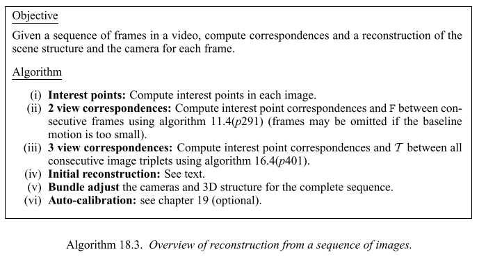
A clear implementation is from cs231a. Assuming camera parameter is known and fixed, each 2view for 0 to 1, 1 to 2, 2 to 3 etc, with the mathcing points, solve 2view to get motion and 3d points. Then merge to get 0 to 2, then 0 to 3 etc. By first transform 2 to 3 frame to 0 frame’s coordindate system (the motion and 3d structure). Adding new 3d point and its projection from last two images. Then trianglate to adjust all 3d points across all images, then bundle adjust motions and structures together. The matches here are sparse like 50 points per image. Final 3d point cloud is from pairwise dense image match, eg 30k points per image pair, trianglate using the accurate camera motion. now the motion is from frame 0. The 3d points are in terms of frame 0.
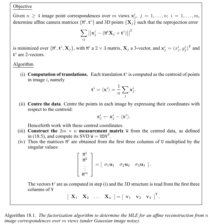
Affine Reconstruction
Define
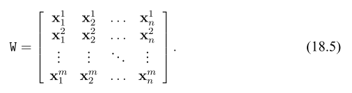 The Affine reconstruction algorithm 18.1 is