Machine Learning A Probabilistic Perspective

02 Jun 2018

Machine Learning: A Probabilistic Perspective by Kevin P. Murphy is a comprehensive book covering many topics on machine learning. In this blog, I will try to summarize things that I find important.

• Preliminaries
  • Probabilities
  • Discrete Generative Models
  • Gaussian
  • Bayesian statistics
  • EM
• Linear Models
  • Linear regression
  • Logistic regression
  • GLM
  • Latent Linear Models
  • Sparse Linear Models
• Nonlinear Models
  • Kernels
  • Gaussian Process
  • Decision Trees and Boosting
• Graphical Models
  • Bayes Nets
  • HMM
  • State Space Models
  • Markov Random Fields
  • Exact Inference for Graphical Models
  • Monte Carlo Inference
• Clustering

Preliminaries

Probabilities

$$\begin{matrix} p(X=x \mid Y=y) & = & \frac{p(X=x) p(Y=y \mid X=x)}{\Sigma_{x'} p(X=x') p(Y=y \mid X=x')} \\ Bin(k\mid n, \theta) & \triangleq & \binom{n}{k} \theta^k (1-\theta)^{n-k} \\ Beta(x\mid a, b) & Y & \frac{1}{B(a, b)} x^{a-1} (1-x)^{b-1} \\ Mu(x\mid n, \theta) & \triangleq & \binom{n}{x_1 \dots x_K} \prod\limits_{j=1}^{K} \theta_j^{x_j} \\ Dir(x\mid \alpha) & \triangleq & \frac{1}{B(\alpha)} \prod\limits_{k=1}^K x_k^{a_k -1} \mathbb{I}(x\in S_K) \\ \mathit{N}(x \mid \mu, \Sigma) & \triangleq & \frac{1}{(2\pi)^{D/2} \lvert \Sigma \rvert^{1/2}} exp [-\frac{1}{2} (x-\mu)^T \Sigma^{-1} (x-\mu)] \\ \mathbb{H}(X) & \triangleq & -\sum\limits_{k=1}^K p(X= k) \log_2 p(X=k) \\ \mathbb{KL}(p \parallel q) & \triangleq & \sum\limits_{k=1}^K p_k \log\frac{p_k}{q_k} \\ \mathbb{I}(X;Y) & \triangleq & \mathbb{KL}(p(X, Y) \parallel p(X)p(Y)) \end{matrix}$$

Discrete Generative Models

beta-binomail model: $p(\theta \mid D) \propto Bin(N_1 \mid \theta, N_0 + N_1) Beta(\theta\mid a, b) \propto Beta(\theta \mid N_1+a, N_0+b)$.

Dirichlet - multinomial model: $p(\theta\mid D) \propto Dir(\theta\mid \alpha_1+N_1, \dots, \alpha_K+N_K)$

logsumexp trick: factor out largest term.

Bayesian naive Bayes for binary features, $N_c$ is the num of docs belongs to class $c$, $N_{jc}$ is the num of docs in class $c$ where word $j$ appears. 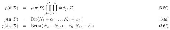For prediction, use the mean get same result using full Bayesian prediction Naive bayes can also use multinomial model, where words appearance are counted.

Gaussian

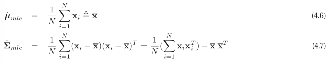
MLE of MVN

GDA, LDA: $p(y=c \mid x, \theta)$ where $p(x \mid y=c, \theta)$ is gaussian, LDA tie $\Sigma_c = \Sigma$

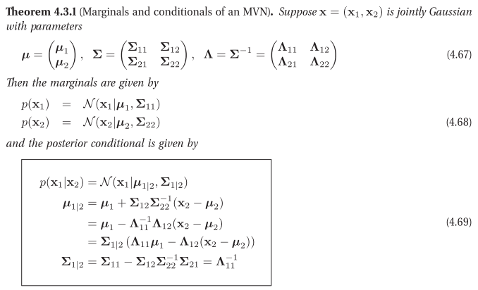
Marginal and conditional

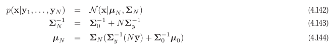
posterior of Gaussian after noisy measurement is also a Gaussian.

Posterior $p(\mu, \Sigma \mid D)$ of mean and variance is Normal-inverse-wishart (NIW) distribution.

Bayesian statistics

In frequentist statistics, data is random, parameter is viewed as fixed. Estimate $\hat{\delta}$ is computed by an estimator $\delta$, so $\hat{\theta} = \delta(D)$. Bootstrap can compute the sampling distribution. Use cross validation to esitmate risk of estimator. Estimator selection can be guided by the bias-variance tradeoff.

Bayesian statistics concepts:

• prior $p(\theta)$
• posterior $p(\theta \mid D)
• MAP $\hat{\theta} = arg\max p(\theta\mid D)$
• credible intervals: sample the posterior
• posteiror predictive density $p(x\mid D)$

Bayesian model selection select model $\hat{m} = argmax p(m \mid D)$, assuming uniform prior over models, then pick model maximize marginal likelihood for model $m$. $p(D\mid m) = \int p(D\mid \theta) p(\theta\mid m) d\theta$. Interestingly, models with more parameters may not have higher marginal likelihood. One approximation is Bayesian information criterion (BIC) $BIC \triangleq \log p(D\mid \hat{\theta}) - \frac{dof(\hat{\theta})}{2} \log N$. dof is the number of parameters of the model.

Classification metrics:

• true positive rate: $TPR = TP / N_{+}$
• false positive rate: $FPR = FP / N_{-}$
• ROC curve: x is FPR, y is TPR by reducing threshold.
• precision-recall curve: y is precision $TP/\hat{N}_{+}$, x is recall, ie true positive rate.
• F score: $F_1 \triangleq \frac{2}{1/precision + 1 / recall}$

EM

Advantages of latent variable are: reduce num of parameters; serve as bottlenecks. Discrete latent state: $p(x_i \mid \theta) = \sum_{k=1}^K \pi_k p_k(x_i \mid \theta)$. EM has two steps:

• E step, infering missing values given parameters, compute expected complete data log likelihood $Q(\theta, \theta^{t-1}) = E[l_c(\theta) \mid D, \theta^{t-1}]$.
• M step, optimizing parameters given the filled in data. $\theta_t = arg \max\limits_{\theta} Q(\theta, \theta^{t-1})$

Examples:

• GMM: parameter is $\pi_k, \mu_k, \Sigma_k$.
• k-means is a speical GMM where covariance is diagnal, and the cluster assignment is hard.

Linear Models

Linear regression

$p(y\mid x, \theta) = N(y \mid w^T x, \sigma^2)$

Graident of NLL is $g(w) = [X^T X w - X^T y] = \sum\limits_{i=1}^N x_i (w^T x_i - y_i)$, the MLE is $\hat{w}_{OLS} = (X^T X)^{-1} X^T y$

convex function’s Hessian is positive definite. NLL is negative log likelihood. max likelihood is min of NLL. Huber loss is a combination of $l_1$ and $l_2$ loss, is C1 smooth, gradient is the same.

There is a choice of likelihood and prior for linear regression on table 7.1. Ridge: gaussian + gaussian prior. Lasso: gaussian + laplace prior. Robust regression: Laplace (or student). but objective function is not smooth. Better to use (Gaussian + Huber loss). Ridge regression: l2 regularization, gaussian prior on w. $w = (\lambda I_D + (X^T X))^{-1} X^T y$

one way to deal with b is to center output $y - \bar{y}$. For Bayesian linear regression, the posterior on w is also guassian, the predictive density is also gaussian, the variance dependes on x. With more data, variance of $w$ is reduced. When given x is far from data, the prediction is more unsure. This is important for active learning.

Logistic regression

$p(y \mid x, w) = Ber(y \mid sigm(w^T x))$ Here $y$ is 0 or 1. Logistic regression no closed form solution, still convex hessian is positive definite. Gradient, Hessian

$$\begin{matrix} g & = & X^T (\mu - y) = \sum_i (\mu_i - y_i) x_i \\ H & = & X^T S X, \ where\ S = diag(\mu_i ( 1 - \mu_i)) \\ w_0 & = & \log(\frac{\bar{y}}{1-\bar{y}}) \end{matrix}$$

It can be solve by iteratively reweighted least squares, where weighting is updated.

Optimization methods:

• Gradient descent: line search is zigzag, because search direction is orthogonal to gradient at endpoint. with momentum $\theta_{k+1} = \theta_k - \eta_k g_k + \mu_k (\theta_k - \theta_{k-1})$
• Conjugate gradient never repeat same search direction, no zigzag. It will find orthogonal direction for the Hessian (ie unwarp it).
• Newton method fit a qudratic around x_k: solve $H_k d_k = -g_k$, ie $d_k = - H_k^{-1} g_k$ then use line search to find $\eta_k$. If H_k is not postive definite (ie function is non convex), $d_k$ may not be decreasing. In this case, can set $d_k = -g_k$. This is Levenberg Marquardt.
• Quasi-Newton: maintain a low rank approximation of $H_k$ is BFGS. In L-BFGS, the approximation is about 20 pair of vectors $(s_k, y_k)$, and $H_k^{-1} g_k$ is approximated by these pairs.
• Adagrad: gradient descent step size divide by sum of squares of graident per parameter.

multi-class (multinomial) logistic regression (maximum entropy classifier): the MLE, NLL is similar to binary one, ie error term multiply $x_i$ $\nabla_{w_c}f(W) = \sigma_i(\mu_{ic} - y_{ic}) x_i$.

Bayesian logistic regression: no conjugate prior, has to approximate posterior. Online learning: objective is regret minimization with given loss function. approach is stochastic gradient descent or bayes filter.

Generative: $\sum \log(p(y_i, x_i))$, discritive $\sum log(p(y_i \mid x_i))$. generative model can handle missing data by introduce a hideen variable to represent if data is missing, then use EM to train. Fisher discriminant analysis is discrimitive. It seeks to find $w$ so that in class variance is small, but between class variance is large. $w = S^{-1}_W(\mu_2 - \mu_1)$, $S^{-1}_W$ is sum of in class variance.

GLM

Exponential family distribution $p(y\mid \eta) = b(y) \exp(\eta^T T(y) - a(\eta))$. $\eta$ is canonical parameter, $T$ is sufficient statistics, $a$ is log partition. Many belongs to exponential family, but student t is not. Ber $p(y; \phi) = \phi^y (1-\phi)^{1-y}$ belongs to exponential family

$ \eta = \log(\phi / (1-\phi)), T(y) = y, a(\eta) = \log(1+e^\eta), b(y) = 1 $

logit function: log(a/(1-a)), inverse is sigmoid (or logistic)

In GLM, the conditional probability is in exponential family. Let $\eta = w^T x$. We want $h(x) = E[T(y)\mid x; \theta]$, in most cases $T(y) = y$. Given these three assumptions, we can derive several learning algorithm.

• Ordinary least Sqaure: $h_{\theta}(x) = E[y \mid x; \theta] = \mu = \eta = \theta^T x$. The reponse function is identity.
• Logistic Regression: $h_\theta(x) = E[y \mid x; \theta] = \phi = 1/(1+e^{-\eta}) = 1/(1+e^{-\theta^T x})$. The response function is logsitic function.
• probit regression: response function is cdf of standard normal.

With GLM, the gradient of NLL to parameter is the familiar formula.

$\triangledown \mathit{l}(w) = 1/\sigma^2 [\sum_{i=1}^N (y_i - h(x_i)) x_i]$

multi-task learning: personalized models, where parameters share same prior. trick: two copies of the feature with and without user_id for spam filter. feature with userid ‘s weight is the delta weight.

Latent Linear Models

Factor analysis: $z$ is gaussian, $y = W z + U + noise$. It is a low rank approximation of MVN. $p(z \mid y)$ is also gaussian. Generate a low dimension $z$, use $w$ to map to high dimension, add noise. Parameter $w$ has a closed form formula. When noise has variance $\sigma^2 I$, this is called PPCA, $w$ are the principal components.

PCA: Minimize reconstruction error $J(W, Z) = \lVert X - W Z^T\rVert_F^2$, $Z$ is $NxL$. The solu is eigenvectors of the covriance matrix of X. The new coordindate is $\hat{z}_i = W^T x_i$. Standard the data to remove scale.

SVD: $X = U S V^T$, U is NxN, S is NxD, V is DxD. columns of U is left, columns of V is right eigenvector. Principal vectors $\hat{W} = V$, $\hat{Z} = X \hat{W}$.

PCA for categorical data: use the factor analysis formulation, except $y$ is not normal given z, but multinoulli with mean softmax of $w z$. No closed form solution, use EM to solve this.

Sparse Linear Models

Make W has a lot of zeros. Bayesian variable selection $\gamma$ is the bitvector for selected features, $p(\gamma \mid D)$ is a softmax of a cost function over all $2^{\lvert \gamma \rvert}$ bitvectors. In practice use greedy search.

feature selection $\gamma$ can be fomulated as optimizing the posteior $p(\gamma \mid D)$, then need to integrate out the fitted weights $w$ and their variance. There are two model of $w$, one is the spike and slab model, the other is binary mask model. The latter leads to $l_0$ regularization (num of non zeros). $f(w) = \lVert y - xW\rVert_2^2 + \lambda \lVert w \rVert_0$

l1 regularization: assume laplace prior on $w$, then $f(w) = NLL(w) + \lambda \lVert w \rVert_1$ for linear regression, become lasso, shows it has sparse solution geometrically $min_w RSS(w)\ s.t. \lVert w \rVert_1 \leq B$ still convex.

subgradient or subderivative for absolution function at 0 is a [-1, 1], which includes 0. $\hat{\theta}$ is a local minimum of $f$ iff $0 \in \delta f(\theta) \mid \hat{\theta}$. With ridge shrink $(1+\lambda)$, for lasso, it is soft thresholding.

Nonlinear Models

Kernels

Kernel helps to create non linear models. $k_{ij} = \phi(x_i)^T \phi(x_j) \geq 0$ measure similarity between objects. A kernel is a Mercer kernel iff the Gram matrix any set of inputs is positive definite.

• RBF
• cosine similarity (use raw count, or tf-idf)
• string kernel: common substrings.

GLM with kernel: kernal machine $\phi(x) = [k(x, u_1), dots, k(x, u_k)]$. If use data itself as $u_i$ then use sparse model: L1VM, RVM (sparse model by ARD/SBL)

kenel trick: provided algorithm can be use $x^T x$ instead of $x$.

svm for regression: epsilon insensitive loss function, within $\epsilon$ loss is zero. Add slack variable, solve by quadratic programing. $\hat(y) = \hat{w}_0 + (\sum_i \alpha_i x_i)^T x$.

svm for classification: $y \in {0, 1}$, hinge loss. objective is $min_{w,w_0} 1/2 \lVert w \rVert^2 + C \sum(1-y_i f(x_i))_{+}$. Use linear svm for large problem, for non linear, use SMO or QP solvers on the dual problem. $\hat{w} = \sum \alpha_i x_i$, $\hat{y}(x) = sgn(\hat{y_0} + \hat{w}^T x)$

smv output to probability: use output of svm as log odds ratio, train a separate 1d logistic regression on another dataset: $p(y=1\mid x) = \sigma(a f(x) + b)$. Platt. not well calibrarated.

multiclass logistic regression is easy. for svm is hard, train one-vs-all (see which class has max output). one-vs-one (then see which class get most vote).

Should use RVM or GP, SVM is not the best.

Other kenel models:

• kernel density estimation (KDE) $p(x) = 1/N \sum k_h(x - x_i)$
• kernel regression $f(x) = \sum w_i(x) y_i, w_i(x) = \frac{k_h(x-x_i)}{\sum k_h(x-x_{i’})}$ weighted sum of training data.
• locally weighted regression: weight is $k(x, x_i)$.

Gaussian Process

GP has a mean function and a kernel function, it is a distribution over functions, each function is a MVN at any finite set of x. $p(f(x1), \dots, f(x_N))$ is gaussian. coverance $\Sigma_{i,j}$ is $k(x_i, x_j)$. The likelihood of a particular function is just the probability of the mvn at these finite points.

GP regression: $y = f(x) + \epsilon$, $f(x)$ is a GP. With a given mean and a correlation kernel, then prediction is a conditional gaussian in closed form formula. The choice of kernel and parameter is important. Here the mean function is 0. Parameters fit by maximize $p(y \mid X) = \int p(y\mid f, X) p (f\mid X) df$.

GP classification. $p(y_i=1 \mid x_i) = \sigma(f(x_i))$. $\sigma$ is the sigmoid function. Need approximation, because Gaussian prior is not conjugate to Bernoulli. maximize posterior of $f$.

Decision Trees and Boosting

Learn the features and weights together.

Classification and regression trees (CART):

• For regression, leaves store mean response. The cost of a tree node is response variable variance $\sum (y_i -\bar{y})^2$, or fit a linear regression model using all previous split variables and measure RSS.
• For classfication, leaves store distributions of each class. The cost of a node is by measuring $y_i$’s entropy or Gini index, which is the expected error rate.
• For missing input, add missing value as a new value; or find highly correlated variables to backup.
• random forrest: reduce variance, bagging.

Boosting:

• fit weighted data by weak learners. boosted decision trees can produce well calibrated proabilities.
• adding next model to minimize the loss, turn out to be weighting each original data.
• logitboost is better than adaboost (put exponetial weight on outliers)
• graident boosting: evaluate loss function gradient for current model, fit this gradient, update model.

Ensemble learning: use cross validation to learn the weights of different models. error correcting output codes is a way to do multiclass, so that each class has max hamming distance.

Comparisions of models:

• For low dimensional data, boosted decision trees is best, logsitic regression and naive bayes the worst.
• For high dimensinal small amount of data, MLP is best, boosted tree is also good.

Feature importance test:

• only used one feature to do predication for the mean averaging over all other variables.
• num of times used in random forrest.

Graphical Models

Bayes Nets

Concepts:

• clique: is a set of nodes that are all neighbors in an undirected graph.
• DAG has a topological ordering.
• bayes net: $p(x_{1:V} \mid G = \Pi_{t=1}^V p (x_t \mid x_{pa(t)})$
• HMM: transition model, observation model
• example: alarm network is a probabilistic expert system
• sigmoid belief net: DGM where CPD are logistic regression
• inference: estimate unknown from known quantities. eg the hidden variables
• learning: comptue MAP estimate of the parameters given data
• plate notation: iid repeated N times
• learning: complete data in DGM, has factored posterior. just counts, add Dirchelet prior.
• $I(G) \subset I(p)$ is an I-map, if graph does not make independence statement not true of $p$. minimal I-map.
• d-separation: undirected path P is d-separated by nodes E.
  • E is in the chain, at the fork, or none of E or descents are at a collider.
  • $x_A \bot_G x_B \iff A is d-separated from B given E$
  • explaining away: condition on a common child makes its parents become dependent.
• conditional indenpdence $t \bot [nd(t) \setminus pa(t)] \mid pa(t)$
• Markov blanket: it makes a node indepdent of all other nodes given the blanket. includes parents, children and co-parents.

HMM

Markov model:

• For language model through counting, deleted interpolation: if $f_{jk}= N_{jk}/N_j$ and unigram frequencies $f_k = N_k/N$, then $ A_{jk} = (1-\lambda)f_{jk} + \lambda f_k$.
• unknown words replace it with special symbol $unk$, held aside some probability.
• stationary distribution is eigenvector for eigenvalue 1. $A^Tv = v$. Every irreduble aperiodic finite state Markov chain has a unique stationary distribution. If $\phi$ satisfied detailed balance for transition matrix $A$, then $\pi$ is the stationary distribution. $\pi_i A_{ij}= \pi_j A_{ji}$.
• power method: repeated matrix vector multiplication followed by normalization to calculate leading eigenvector.

HMM applications include speech, activity recognition, part of speech tagging. CRF maybe more suitable for this, it is dicriminative.

Inference problems in HMM:

• filter: estimate current state given all previous outputs, $p(z_t = j \mid x_{1:t})$. Why called filter? because it reduced noise by calculating $p(z_t\mid x_{1:t})$, insteacd of just $p(z_t \mid x_t)$
• smoothing is $p(z_t \mid x_{1:T})$
• prediction $p(z_{t+h} \mid x_{1:t})$
• MAP estimation: $arg\max_{z_{1:T}} p(z_{1:T} \mid x_{1:T})$ using Viterbi decoding. Smoothing with thresholding should be more accurate than Viterbi?
• probability of evidence $p(x_{1:T})$.

Algorithms:

• forward: used for filtering and probability of evidence. predict-update $\alpha_t \propto p(z_t \mid x_{1:t}) = \phi_t \odot (\psi^T \alpha_{t-1})$. $\phi$ is the output, $\psi$ is the transition. Also used to compute probability of evidence.

• backward: calculate $\beta_t(j) = p(x_{t+1:T} \mid z_t = j)$, ie the future evidence conditioned on current state. $\beta_{t-1} = \psi(\phi \odot \beta_t)$
• smoothing: $\gamma_t(j) = p(z_t = j \mid x_{1:T}) = \alpha_t(j) \beta_t(j)$.

• two-slice smoothed marginal: expected $N_{ij} \mid x_{1:T}$ is $\xi_{t, t+1}(i, j) = \alpha_t(i) \phi_{t+1}(j) \beta_{t+1}(j) \psi(i, j)$

• Viterbi: shortest path on the trellis diagram. recursive step is compute the max proability of a prefix ends up in state j. For multiple path, can sample from posterior using two sliced marginal.

EM for HMM (Baum-Welch): expected complete data likelihood, use forward backward to estimate state and transitions for each sequence. Estimate the proability of latent variables of each step of each sequence, eg $\gamma_{i,t}$, the transition and output distribution can be maximized in M step. EM can be further improved by discrimitive training.

State Space Models

SSM is HMM with continuous hidden states. LG-SSM: linear gaussian ssm: for tracking, SLAM.

$$\begin{matrix} z_t = g(u_t, z_{t-1}, \epsilon_t) \\ y_t = h(z_t, u_t, \delta_t) \end{matrix}$$

The presentation of kalman filter, EKF, UKF are similar to the “Probabilistic Robotics” book. kalman smoothing algorithm: offline, similar to forward and backward of HMM.

learning SSM: fully observable, then use linear regression to fit z and y. EM for partial observable. hybrid discrete/continuous SSMs: $q_t$ discrete state, $z_t$ continuous state, $y_t$ is measurement. Applications: data association, econometric forecasting.

Markov Random Fields

Markov blanket is the node’s neighbors. Normalization to convert DGM to UGM add more edges due to common children, but introduce more dependences at other places. Neither is more powerful than the other. One factor per max clique. $p(y\mid \theta) = \frac{1}{Z(\theta)} \prod_{c\in C} \psi_c(y_c\mid \theta_c)$. Log-linear model $\log(p(y\mid \theta)) = \sum_c \phi_c(y_c)^T \theta_c - Z(\theta)$

Examples:

• Ising model: $w_{st}$ is weight between two nodes, $log p(y) = - y^T W y$.
• Hopfield networks: associate memory for bitvectors, inference by coordinate descent
• Boltzmann machine: has latent variables.
• Potts model: clustering for image segmantation
• Guassian MRFs

Learning:

• log linear MRF by moment matching $\frac{\delta l}{\delta \theta_c} = [1/N \sum_i \phi_c(y_i)] - E[\phi_c(y)]$
• With hidden variable by marginalize over $h_i$ $\frac{\delta l}{\delta \theta_c} = [1/N \sum_i { E[\phi_c(h, y_i) \mid \theta] - E[\phi_c(h, y)\mid \theta]}$
• Stochastic maximum likelihood: in each gradient descent step, use current $\theta$ to sample $y_c$ use the mean to be the expectation.

CRF is discrimitive, one application is disparity in stereo. It is offline, not for real time applications.

• $p(y\mid x, w) =1/Z(x, w) \prod_c exp(w_c^T \phi(x, y_c)$
• learning $\frac{\delta l}{\delta \theta_c} = 1/N \sum_i [\phi_c(y_i, x_i)] - E[\phi_c(y, x_i)]$. For each input instance x_i, need to estimate the expected model output, can’t share one across minibatch. $w$ is shared, so the features are sumed acroos all node and edge before multiplying with $w$.

RBM: product of experts, visble and hidden form a bipartite graph. $p(h, v\mid \theta) = \frac{1}{Z(\theta)} \prod_{r=1}^R \prod_{k=1}^K \psi_{rk}(v_r, h_k)$. Use contrastive divergence algorithm to approximate gradient. $\frac{\delta l}{\delta w_{rk}} = \frac{1}{N} \sum_{i=1}^N E[v_r h_k \mid v_i, \theta] - E[v_r h_k \mid \theta]$

hierarical classification: toxonomy tree, an instance’s y has multiple bits turns on.

Exact Inference for Graphical Models

For direct and undirect graphical models with hiden variables, generalize forward/backward algorithm:

• BP for trees: forward path is propagate belief from leaves to root, backward phase is from root to leaves. It is sum of product. calculate the messages on the edges. can do parallel update.
• variable elimination for arbitrary graphs:
• junction tree: generalize bp to arbitrary graphs.

Monte Carlo Inference

Sample distributions:

• use CDF to sample: if $U \sim U(0,1)$ is a uniform rv, then $F^{-1}(U) \sim F$.
• Box-Muller to sample from 1d guassian (change of variables trick), use $y = Lx + \mu$ ,where $\sigma = L L^T$ through Cholesky decomposition.
• rejection sample: $M q(x) \geq \tilde{p}(x)$, $q$ is proposal, sample $x \sim q(x)$ accept if $u > \frac{\tilde{p}(x)}{M q(x)}$, where $u \sim U(0, 1)$.
• importance sample: to compute $E[f]$ for $p(x)$, then sample from $q(x) and calulate $1/S \sum f(x) p(x)/q(x)$
• mcmc constructs a Markov chain whose stationary distibution is $p^{*}(x)$, then sample from this chain. Burn in to let the chain forget where it starts.
  • Gibbs sampling: sample $p(x_i \mid x_{-i})$, eg ising model, percentage of neighbors in each state.
  • Metropolis Hastings algorithm: propose $q(x’ \mid x)$, accept with probability \frac{p^{}(x’) / q(x’ \mid x)}{p^{}(x) / q(x \mid x’)} This actuall make sure visit each state $x$ based on probability $p^{*}(x)$.

Clustering

clustering metrics: purity: average accuracy across clusters based on labels

spectral clustering: $W$ is the distance matrix, $D$ is a diagonal equal to sum of each row of $W$, Graph Laplacian $L \triangleq D - W$, it is positive semi-definite. Compute $K$ smallest eigenvector of $L$ to become matrix $Y_{NxK}$ take the $N$ rows and perform k-means on them. Assign point $i$ to cluster $k$ iff row $i$ of $Y$ was assigned to cluster $k$.

hierarchical clustering:

• agglomerative (bottom-up) dendrogram, single link (minimum spanning tree), complete link, average link
• divisive (top-down), choose a cluster to bisect, eg using k-means with 2 cluster
• Bayesian hierarchical clustering by measure probability of merging to clusters $ r_{i,j} \triangleq \frac{p(D_{ij} \mid M_{ij} = 1) p (M_{ij} = 1)}{p(D_{ij} \mid T_{ij})} $