Probabilistic Robotics
27 Aug 2018Probabilistic Robotis by Sebastian Thrun, Wolfram Burgard and Dieter Fox is a great book. I decied to read it after taking the Artificial Intelligence for Robotics Udacity class. Here I am going to summary the main things I learnt from the book. All the included figures are blatantly copied from the book.
First of all, this book is mainly about mobile robots SLAM on a 2d plane. The pose is $x, y, \theta$, the map can be occupancy grid maps or feature based (landmarks) maps. The last part of the book is about planning, ie policy for achieving a goal state.
Preliminary
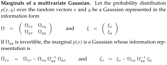
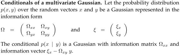
Gaussian marginalization and conditional in information matrix:
Motion models
Velocity model
The first motion model is velocity model($v, \omega$) for a circular movement in a small time $\Delta t $.
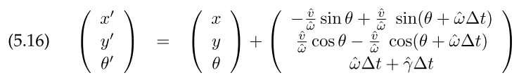 The $\hat{v}, \hat{w}, \hat{\gamma}$ includes gaussian noise, $\hat{\gamma}$ is used to model final orientation not accounted for by circular motion. Algorithm motion_model_velocity($x_t, u_t, x_{t-1}$) in Table 5.1 computing $p(x_t | \mu_t, x_{t-1})$ by solving the inverse motion model. Algorithm sample_motion_model_velocity($u_t, x_{t-1}$) in Table 5.2 samples the next pose $x_t$.
Odometry model
The second motion model is odometry model with $\delta_{rot1}, \delta_{trans}, \delta_{rot2}$ from odometry data
\[\begin{align} x^{'} = x + \delta_{trans} \cos(\theta + \delta_{rot1}) \\ y^{'} = y + \delta_{trans} \sin(\theta + \delta_{rot1}) \\ \theta^{'} = \theta + \delta_{rot1} + \delta_{rot2} \end{align}\]Bicycle model
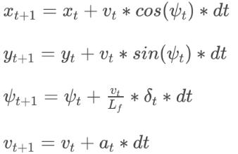
The third motion model is bicycle model with length. The move function calculate new pos given current pos and steering angle and rear wheel travel distance.
def move(self, x, y, orientation, steering, distance):
  radius = length / np.tan(steering)
  turn = distance / radius
  cx = x - (np.sin(orientation) * radius)
  cy = y + (np.cos(orientation) * radius)
  norientation = (orientation + turn) % (2.0 * np.pi)
  nx = cx + (np.sin(self.orientation) * radius)
  ny = cy - (np.cos(self.orientation) * radius)
  return nx, ny, norientation
If the input is acceleration and steering, use this model
Range Sensor model
Given map $m$, robot pose $x_t$ at time t, compute the probability $p(z_t \mid x_t, m)$ for measurement $z_t$. Here only consider 2d range scanners, eg sonar and laser, so $z_t$ is a distance measurement.
Beam model
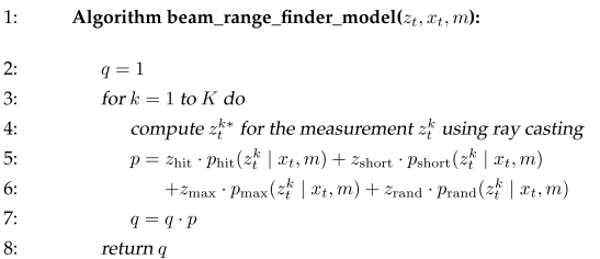
Assume multiple measuremnt in the same scan is indepdenent. $p(z^k_t \mid x_t, m)$ is a mixture of four models: Gaussian $p_{hit}$, exponential $p_{short}$, uniform $p_{max}$ and uniform $p_{rand}$. Let $z_t^{k*}$ to denote the true range of the object measured by $z^k_t$. It is obtained by ray casting. The internal parameters of each model and the mixing weight can be computed via an EM algorithm learn_intrinsic_parameters in Table 6.2. With the parameters, algorithm beam_range_finder_model($z_t, x_t, m$) compute the likelihood of a range scan $z_t$. To make this efficient, can calculate a subset of measurements per scan, can also precashing ray casting algorithm by discretizing $x_t$.
Landmark Model
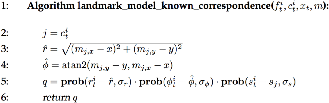
Each landmark has a location, its measurement has range, bearing and a signature.
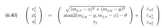 Given one landmark measurement, the posterior of robot pose is given in algorithm sample_landmark_model_known_correspondence($r_t^i, \phi_t^i, c_t^i, m$).
Occupancy Grid Mapping
Given known pose (eg after slam) construct occupuancy maps from noisy range measurements. This is alsoc alled inverse measurement models. The likelihood of occupancy is represented by log odds. For each measurement, all grid cells in the field of view are considered and their likelihood is adjusted by the inverse sensor model.
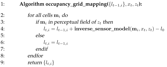
Cells close to the measured range is assigned high likelihood $l_{occ}$, shorter ones are free, and longer ones no change. $\alpha$ is obstacle depth, $\beta$ is openning angle of the beam. Machine learning can be applied to learn this model.
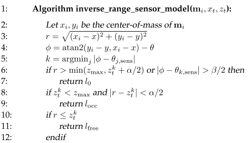
Mapping can also use forward model: select the occupancy that maximize the measurement.
Bayes Filters
Recursively estimate robot state through motion and measurement update.
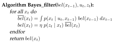 Using $\eta$ to represent normalization.
Histogram Filter is discretized version, and applied for low dimentional state space. The decomposition can be metric regularly spaced grids or topological with significant places. Dynamic density tree is used to dynamically adjust decomposition resolution.
Using $\eta$ to represent normalization.
Histogram Filter is discretized version, and applied for low dimentional state space. The decomposition can be metric regularly spaced grids or topological with significant places. Dynamic density tree is used to dynamically adjust decomposition resolution.
Kalman Filter
Linear Gaussian system repersents states by Gaussian. $x_t = A_t x_{t-1} + B_t u_t + \epsilon_t$, $z_t = C_t x_t + \delta_t$.
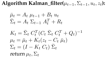 Measure update derivation is by rewriting product of two gaussian into a gaussian. For the quadratic form, take first and second derivative. Second derivative become inverse of final variance. The final mean is by taking zero of the first derivative. Intuitively Kalman gain $K_t$ represents the ratio between variance from motion and variance from measurement. The final mean is shifted by this ratio between measurement mean and post motion mean. The motion variance is reduced by this ratio.
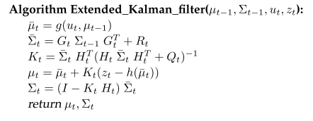
If the state transition and measurement function is not linear, one can use linearize these function at the mean $\mu_{t-1}$ and post-motion mean $\hat{\mu}_t$. The resulting algorithm is called Extended Kalman Filter.
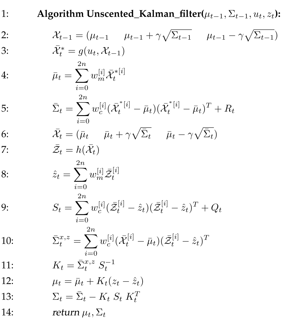
Unscented Kalman Filter use sigmapoints perform linearization. It is amazing that 2n+1 samples can accurate represents post-motion state mean and variance (Line 2 to 5). A similar linearization is used to calculate mean and variance of the expected measurement gaussian (Line 6 to 9). Line 10 is cross-covariance of state and measurement. Line 11 is kalman gain. Line 12 and 13 are the final mean and variance.
Information filter is the dual of Kalman filter, it uses canonical instead of moments parameterization $\Omega = \Sigma^{-1}$ and $\xi = \Sigma^{-1} \mu$. Extended information filter is the dual of Extended Kalman filter.
Particle Filter
In Particle Filter, belief is represented by a set of particles. The regions with dense particles have higher beliefs.
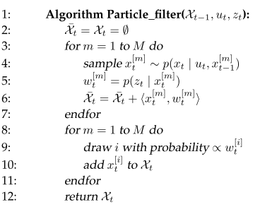 Particle filter uses importance sampling: $f$ is target, $g$ is proposal, requires $f > 0 \rightarrow g > 0$. Repeted resampling can cause low diverity and particle deprivation. One efficient weighted sample algorithm is Walker’s alias method.
Localization
Three flavors of localization with increasing difficulty: local, global and kidnapped robot (teletransport). Filter sensor measurement to deal with unmodeld dynamics. Localization assumes map exists. Here we will use a velocity model and feature maps. It is direct application of Bayes Filter. The EKF localization algorithm is shown to demonstate the linearization for velocity and measture model.
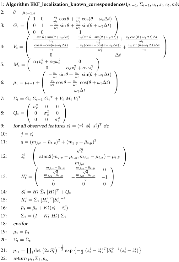 Line 6 is the velocity motion model, except there is no $\gamma$ here. Line 7 is the post motion variances by linearizing motion model at pose $\mu_{t-1}$ and control $u_t$. Line 3 is the jacobian to $\mu_{t-1}$, and Line 4 is the jacobian to $u_t$. Line 8 is the prior variance of feature based landmark sensor model $r, \phi, s$. Line 9 is a loop to incoroprate each landmark since they are independent. Line 12 is the expected measurement. Line 13 is the jacobian of measurement to $\bar{\mu_t}$. Line 14 is the expected measurement variance. Line 14, 15 and 16 is measurement update. Line 21 is the total measurement likelihood. One question is whether the result depdends on the order of update? Since later update builts on top of updated Gaussian, it looks like the result is order dependent. Similary for the total measurement likelihood.
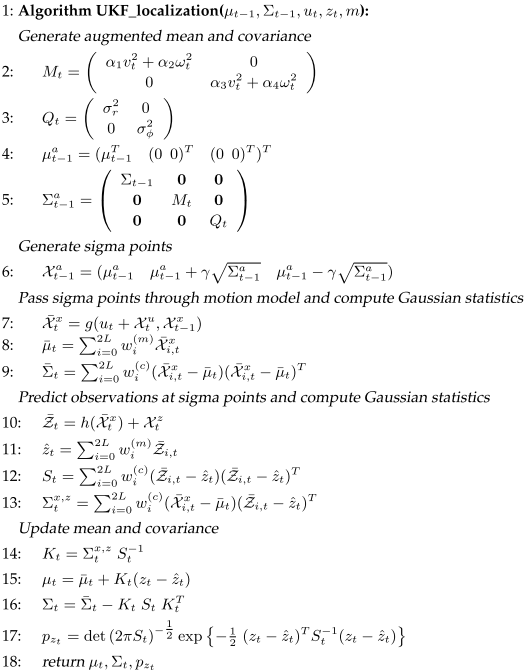
The UKF localization algorithm is similar to before, except here using an augmented state so that sigmapoint has $x_{t-1}, u_t, z_t$. Each component is then used seperately.
For feature based maps, there is always the correspondence issue. Given robot pose, if the feature for a measure is known, then the likelihood of obtaining this measure is calculated as in Line 21. With known correspondence, for each measurement, the feature with maximum likelihood is chosen. There is also an approach called multi-hypothesis tracking (MHT) by mixing of Gaussian where each has a particular set of correspondences.
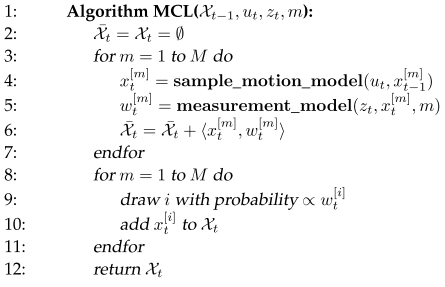
Particle filter (MCL) is great at localization. Inject random particles to deal with global and kipnapped robot. Augmented algorithm adds random particles if sum of total weights of particles are dropping fast. KLD-sample dynamic adjusts num of particles by measuring how widespread current set of particles is.
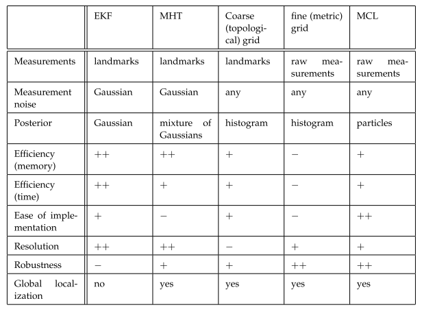
Comparision of common localization algorithms.
SLAM
online SLAM only the last pose. full SLAM estimate the full path.
EKF online SLAM
Use feature based maps (landmarks). Trick is to enlarge state vector to include all landmarks. With motion, variance matrix increases. Until robot sees the initial landmark again, it localized itself and all landmarks. The covariance matrix encodes the dependency.
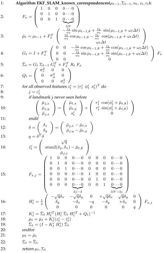 Line 2 to 5 updates the pose mean and variance using motion model. The map mean variance and pose map covariance is kept unchanged. Compared with EKF localiation, here $R_t$ is the same as $V_t M_t V_t^T$ there. Line 16 is the linear model, ie jacobian to both the pose $\bar{\mu_t}$ and feature $\mu_{j}$. At Line 15, the columns for pose and columns for feature $j$ are non-zero. So the update are made to pose and feature j and their covariance at Line 18 and 19. EKF SLAM has quadratic update time in terms of num of features, so it can handle only maps with less than 1,000 features.
With unknown correpondence, again match with maximal likelihood. If all likelihood is small, create a new landmark. Use provisional landmark list for newly introduced landmarks, mantain landmark existence probability to remove false landmarks. Data association is still hard problem. it is no longer the best method.
GraphSLAM
GraphSLAM is invented by Lu and Milios in 1997, their paper has 1141 citations. GraphSLAM is full slam. Intuitively motion and measurement introduce edge in a sparse graph, edges are like springs.
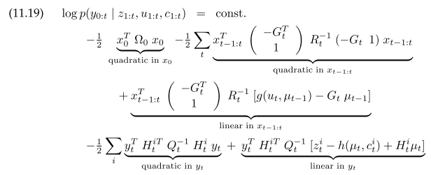
GraphSLAM is similar to EKF, but instead of actively resolving information into covariance matrix, it lazily accumulate information into an information matrix. Using motion and feature sensor model with Gaussian noise, $y_t$ is the augmentated state with all poses and features, the full posterior is
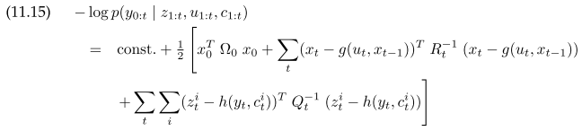 Using EKF style linearization and reorder terms, the log likelihood of the full slam become
 Solving for the $y_{0:t}$ that maximize 11.20 gives $y_{0:t} = \Sigma^{-1} \xi$. To construct $\Sigma$ and $\xi$ directly, for each motion:
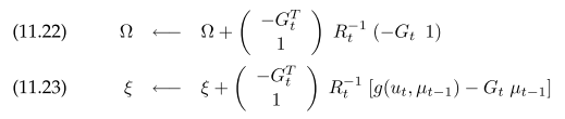 For each measurement
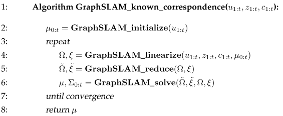
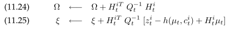 Same as in EKF SLAM, $R_t$ is the $3x3$ variance contribution from motion model, $G_t$ is the $3x3$ jacobian to $\mu_{t-1}$. $\Omega$ is the $6x6$ two adjacent pose. $Q_t$ is the $3x3$ motion noise. $H_t^{i}$ is measurement jacobian to pose and landmark. To take advantage of the sparse graph, instead of solving $y_t$ as a whole, the map variables can be marginalized leaving only pose variables to solve. Afterwards, each landmark can be solved one by one conditioned on connected poses. This results in the following GraphSLAM algorithm, the loop is for better linearization with improved pose estimation.
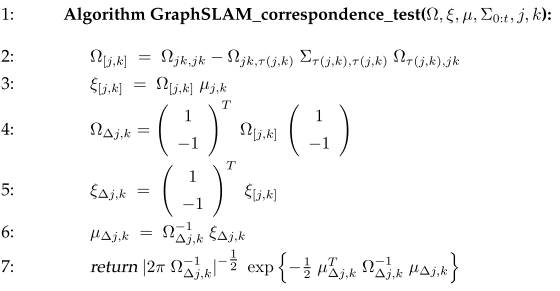
For unknown correspondence, each pair of features are test $j$ $k$ to determine whether they are the same. The likelihood of this is by marginalizing out joint distribution of these two landmarks and calculating the probability of $m_j - m_k$. If this is bigger than a threshold, the GraphSLAM can be repeated incoroporating the new correspondence.
 In practice, features that have high likelihood of correspondence are immediately merged instead of in the end. For example, local occupancy grid maps is used instead of landmarks, matching of two local maps become constraints on poses.
Sparse Extended Information Filter SLAM
SEIF SLAM is similar to EKF SLAM, both are online slam, but SEIF uses information matrix. Its motion update and measurement update are quite similar to the EKF version. What makes SEIF efficient is the sparsification step, which disconnects edges of pose and features by marginalization. By using sparse information matrix, each step of the algorithm takes constant time indepdent of the map size and path length. This sparse approximation makes it less accurate then EKF SLAM and graphSLAM.
SEIF correpondence is similar to GraphSLAM that pair of features are tests to be the same or not: Calculate joint gaussian, then calculate probability of the two feature’s distance in this gaussian. In SEIF, it is easy to add and remove soft links betweeen landmarks with a likelihood estimation, thus a branch and bound algorithm is used. The search tree branches with the maximal likelihood is the final correspondence. This is especially important to demterine loop closures. The information matrix for a soft link is a diagnonal matrix with large diagnoal elements.
multi-robot slam needs to solve correpondence and alignment issues. If known displacement and rotation of the two robot coordindate system is known, one can build a joint information matrix and adding soft constraint to equalize the matching map features by adding a constraint. Correspondence between two robot maps can be achieved by searching for matching local map features.
FastSLAM
Use particle filter, each particle is a sample of path poses and each map feature is repesented by a separate Gaussian. This is because map features are indepndent given a particle which is the path. so it does not need the joint coveriance matrix of EKF. It is also robust to data association problem, each particle makes its own correspondence by maximum likelihood. It solves both full and online slam. It natually deals with occupancy grid maps.
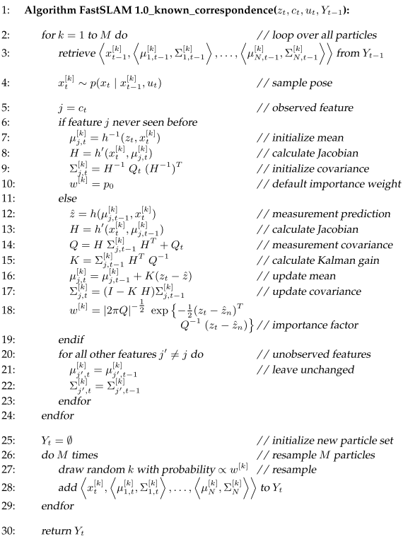 The measurement update is a standard EKF update to each observed feature represented by $\mu_{c_t, t}, \Sigma_{c_t, t}$. The resample weight is the likelihood of the observation. FastSLAM requires $O(M \log N)$, $N$ is size of map. Use tree to represents features of a particle, generating new particles from old one can reuse most of the feature tree that are not observable.
In Fastslam 2.0, proposal distribution also considers measurement, not just motion. It linearizes H, so sample from a gaussian again. The measure update equation and resample weight are more complex gaussians than 1.0.
FastSLAM works for both feature based map and occupancy grid mapss. For grid map, each particle has its path, and the occupancy grid map. For each motion and measurement update, grid map are updated using eg the occupancy_grid_mapping algorithm and weights are calculated.
Planning
Assuming state is observable, but action is uncertain, use MDP to calculate a policy, which maps state to best action, for a given reward function. Th value function of a state satisfies the Bellman equation:
$V(x) = \gamma \, \max\limits_{u} [ r(x, u) + \int V(x’) \, p(x’ \mid u, x) dx’]$
A value function defines the policy
$\pi(x) = arg\max\limits_{u} [ r(x, u) + \int V(x’) \, p(x’ \mid u, x) dx’ ]$
It is common to solve path planning ignoring rotation, velocity etc. To turn such a policy into actual control, need a reactive controller that obeying dynamic constraints. In practice, for low dimensional state space, discretize the state and control space. For high dimensional problem, learning a function. Book has a value function calculation for a 2-DOF robot arm example.
POMDP
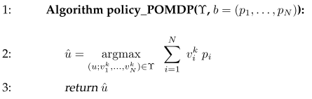
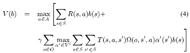
When state is partically observable, planning problem can’t be solve by considerin all possible encironments and averaging the solution. The trick is to use belief to represent the a posterior of the world state distribution. Value function is now over belief. In finite world and finite horizon case, value function is a piece-wise linear function or max of a set of linear function over belief. Given a value funciton $\gamma$ and a belief $b = (p_1, \dots, p_N)$, the policy is calculated by
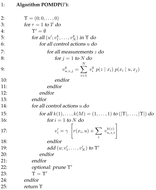
PODMP performs backup loops. In Line 5 to 13, $v_{u, z, j}^k$ is the expected value of at state $j$ take action $u$, get measurement $z$ using the $k$th linear value function. In Line 14 to 21, $(u; v_1^{‘}, \dots, v_N{‘})$ is the value function at step $\tau$, when the $i$th state results in one combination of the next state value functions. The choice can be any combination and the num of choices is num of measurements, so this results in $\mid \gamma \mid^M$ value functions per action. Max pruning is necesary to keep num of linear functions small. An approximation is using point-based value iteration, only consider discrete set of beliefs.
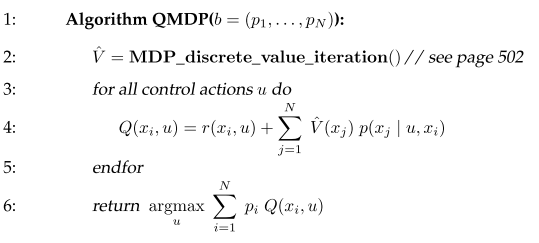
QMDP is an approximate POMDP, it assumes after one step of control, state become fully observable.
AMDP compress belief
\[\bar{b} = \begin{pmatrix} arg\max\limits_{x} b(x) \\ H_b(x)\\ \end{pmatrix}\]It then use MDP value iteration on this augmented state.
MC-POMDP uses particle filter to represent a belief state, can handle non-finite state space. Because each paticle set is unique, this algorithm use nearest neighbor to assign value to a particle set.
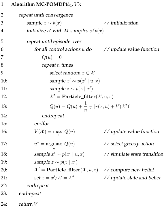 Line 6 to 15 estimates the value of each action for particle set $\chi$, this is done by sampling an action $u$ and oberservation $z$, which are used to compute the next particle set. The best action is chosen and forward simulate to arrive at the next partle set. Which begins the next exploration. In practice, some fraction of random actions is chosen. This is repeated until value function is converged.
SARSOP
The point based POMDP approximation is more popular, eg SARSOP has been used to solve hundreds of states. It is interesting, the author has a paper “point based value iteration: an anytime algorithm for pomdps” on 2003.
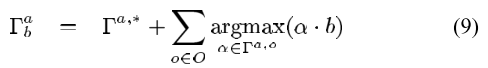
 In pomdp, each output could choose different linear functions. This results in an $\lvert V \rvert = \lvert A\rvert \lvert V^\prime \rvert^{\lvert O\rvert}$ increase in num of functions.
For point based POMDP, each point has a single linear function, value iteration is done over them, because we are calculating the function over a finite set of points, a max is take over existing functions for each belief point. The num of linear function is the same as the num of sampled points.
In pomdp, each output could choose different linear functions. This results in an $\lvert V \rvert = \lvert A\rvert \lvert V^\prime \rvert^{\lvert O\rvert}$ increase in num of functions.
For point based POMDP, each point has a single linear function, value iteration is done over them, because we are calculating the function over a finite set of points, a max is take over existing functions for each belief point. The num of linear function is the same as the num of sampled points.
The SARSOP paper tries to sample point near the reachable state from $b_0$ using the optimal policies by building a search tree starting from initial belief. It uses an underbound and lower bound on optimal value function, and used it to bias sampling. Existing tree branches are removed if it becomes inferior to anothe action. Functions are pruned if it is dominated by others on the sampling points. It can solve POMDP with 15k states in less than 2 hours.
Exploration
In exploration the reward function is a combination of cost and expected information gain. But using this reward function within POMDP is not practical, as the num of observations are large. Here several greedy algorithms are covered. In occupyancy grid mapping, robot moves to its nearest unexplored frontier. For multi-robot, each robot move to the closest unexplored map and prevent others move to vicinity.